B. McCullough - Business Experiments with R
Здесь есть возможность читать онлайн «B. McCullough - Business Experiments with R» — ознакомительный отрывок электронной книги совершенно бесплатно, а после прочтения отрывка купить полную версию. В некоторых случаях можно слушать аудио, скачать через торрент в формате fb2 и присутствует краткое содержание. Жанр: unrecognised, на английском языке. Описание произведения, (предисловие) а так же отзывы посетителей доступны на портале библиотеки ЛибКат.
- Название:Business Experiments with R
- Автор:
- Жанр:
- Год:неизвестен
- ISBN:нет данных
- Рейтинг книги:4 / 5. Голосов: 1
-
Избранное:Добавить в избранное
- Отзывы:
-
Ваша оценка:
Business Experiments with R: краткое содержание, описание и аннотация
Предлагаем к чтению аннотацию, описание, краткое содержание или предисловие (зависит от того, что написал сам автор книги «Business Experiments with R»). Если вы не нашли необходимую информацию о книге — напишите в комментариях, мы постараемся отыскать её.
is an essential resource for any business student. This important text:
Presents the key ideas that business students need to know about experiments Offers a series of examples, focusing on specific business questions Helps develop the ability to frame ill-defined problems and determine what data and types of analysis provide information about each problem Contains supplementary material, such as data sets available to everyone and an instructor-only companion site featuring lecture slides and an answer key Written for students of general business, marketing, and business analytics,
is an important text that helps to answer business questions by highlighting the strategic and technical issues involved in designing experiments that will truly affect organizations.
Business Experiments with R — читать онлайн ознакомительный отрывок
Ниже представлен текст книги, разбитый по страницам. Система сохранения места последней прочитанной страницы, позволяет с удобством читать онлайн бесплатно книгу «Business Experiments with R», без необходимости каждый раз заново искать на чём Вы остановились. Поставьте закладку, и сможете в любой момент перейти на страницу, на которой закончили чтение.
Интервал:
Закладка:
Each trial is so expensive that even a small experiment is too expensive.
The population is too small to support an experiment. There is no point in remodeling a sample of stores to decide whether to remodel the entire population if the population is only 10 stores.
Hypothesis generation is an excellent use of observational data. The researcher explores the observational data looking for interesting ideas that might merit a follow‐up experiment.
Observational data can be used to shed light on causal questions, but the statistical machinery necessary to do so is very sophisticated and still not as good as actually running an experiment. These types of sophisticated analyses are usually performed when an experiment is impossible, not in lieu of an experiment. A standard reference for this type of analysis is Rosenbaum (2010). Using observational data to answer causal questions is hard; so we try to use experimental data, which is comparatively easy.
Notwithstanding the above, it is very common for people to use observational data to (mistakenly) make causal assertions outside of the narrow range in which it can be done. It is very common, therefore, for “causal” results from observational data to be later contradicted by experiments. Many instances can be found in the article by Young and Karr (2011) and the references therein. With respect to establishing causality, unless you are a very skilled statistician, analyzing observational data can only provide what researchers call hypothesis‐generating evidence. In other words, analyzing observational data can give you good ideas for experiments to conduct, but it can't tell you anything about causality.
It is important for the analyst to know whether she has an “umbrella problem” or a “rain dance problem.” If all she wants to know is whether or not she should carry an umbrella, then she has a pure prediction problem and causal questions are of secondary importance; she only needs to know whether the probability of rain is high or low. On the other hand, if there has been a long drought and she wants to end it, prediction is of little value: causal questions are of primary importance. If she wants to induce rainfall, she needs to know what variables cause rain and then try to manipulate those variables. We recall the experience of one analyst, trained in the field of predictive analytics, who had been given some observational data on donations from specific individuals and asked for insight as to whether or not attending fundraisers increased donations. She dropped the variable “number of fundraisers the person attended” because it had no predictive value. She just couldn't understand that her boss had given her a rain dance problem, not an umbrella problem.
Exercises
1 1.1.1 Find an example of an observational study. Answer the following questions: (i) What makes this an observational rather than an experimental study? (be specific) (ii) What is the purpose of the study? (iii) What is the primary variable of interest?
2 1.1.2 For each of the following, indicate whether the data are observational or experimental, and defend your answer.A broadcaster moves a popular television show from Tuesday to Thursday, and its viewership increases.A psychologist wants to know how often students take a break from studying. To do this, he installs cameras in the library's reading room for one day. He notes that students take more breaks in the evening.A sports manufacturer wonders if his quick‐dry exercise shirts dry more quickly than regular shirts. He finds some basketball players playing a game in the gym. He gives one team quick‐dry shirts, and the other team gets regular 100% cotton shirts.A child psychologist asks several parents whether their children play violent video games. He also asks how many times a week their children display violent behavior. He finds that children who play violent video games display more violent behavior.
3 1.1.3 Give two situations where experiments can't be conducted.
1.2 Case: Credit Card Defaults
You work for a credit card company, and you want to figure out which customers might default. In the credit.csvdataset are 30 000 observations on six variables: credit limit (how much can be charged on the credit card), sex of the cardholder, education level of the cardholder (high school, undergrad, grad, other), whether the cardholder is married (single, married, other), the age of the cardholder in years, and whether or not the cardholder defaulted (1 = default, 0 = non‐default).
In this problem we are confronted with the ultimate questions confronting all credit issuers: whether to grant credit to each potential customer and, if so, how much? Generally, we don't want to give credit to people who are likely to default, and if we do give credit, we don't want to give more than the person can repay.
Table 1.1 Credit default rates for men and women.
| Female | Male | |
|---|---|---|
| 0 | 14 349 (79%) | 9 015 (76%) |
| 1 | 3 763 (21%) | 2 873 (24%) |
| Total | 18 112 | 11 888 |
A simple crosstab in Table 1.1with the data shows that men are more likely to default than women. Another crosstab in Table 1.2shows that divorced/widowed (other) persons are more likely to default.
Table 1.2 Credit default rates by marital status.
| Married | Single | Other | |
|---|---|---|---|
| 0 | 10 453 (77%) | 12 623 (79%) | 288 (76%) |
| 1 | 3 206 (23%) | 3 341 (21%) | 89 (24%) |
| Total | 13 659 | 15 964 | 377 |
Try it!
We encourage you to replicate the analysis in this chapter using the data in the file credit.csv. Computing crosstabs can be done in a spreadsheet using pivot tables. Most statistical tools also have a cross‐tabulation function.
df <- read.csv("credit.csv",header=TRUE) # Table 1.1 table1 <- table(df$default,df$sex) # to get the counts table1 # to print out the table prop.table(table1,2) # to get column proportions prop.table(table1,1) # to get row proportions
In addition to the categorical variables in our data set like sex and marital status, we also have continuous variables like age. Perusing the boxplots in Figure 1.2, it appears that persons who do not default have higher credit limits than persons who default, while age appears to have no association with default status.
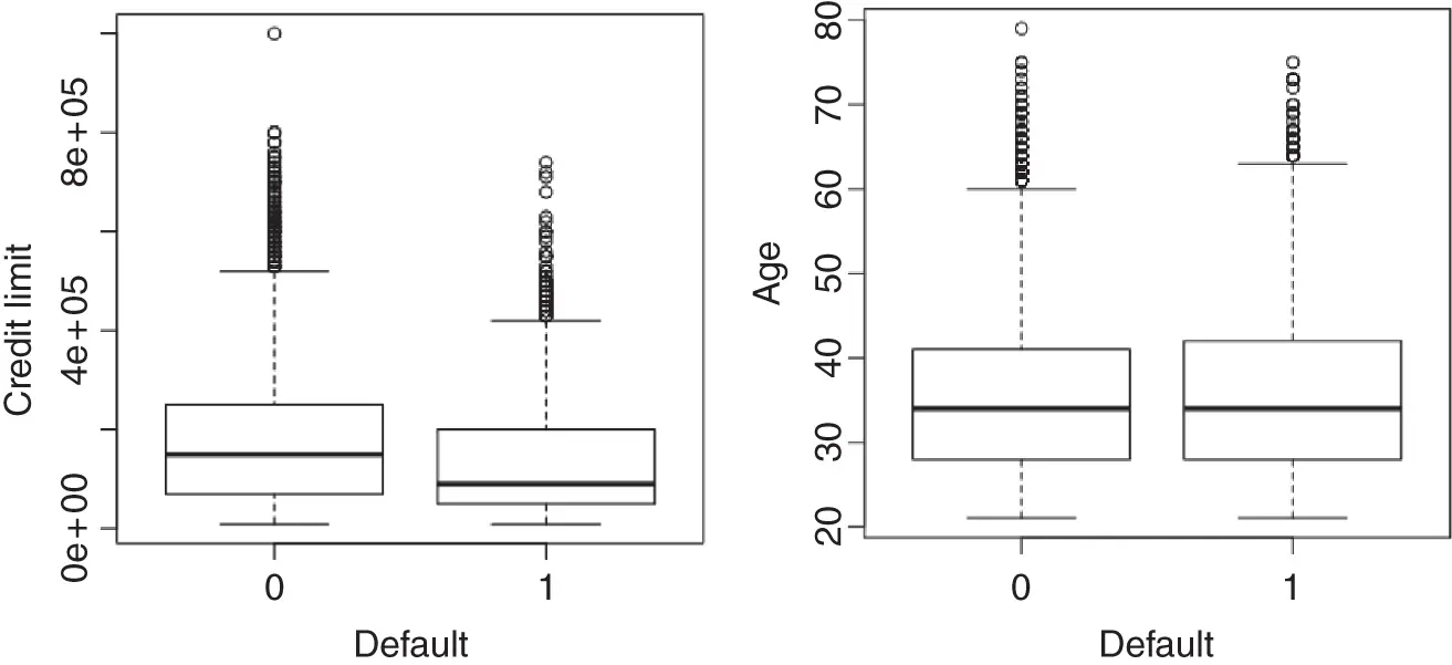
Figure 1.2 Boxplot of default vs. non‐default for credit limit and ages.
If it is really the case that persons with higher credit limits are less likely to default, can we decrease the default rate simply by giving everybody a higher credit limit?
Software Details
To reproduce Figure 1.2, load the data file credit.csv…
boxplot(limit∼default, xlab="default", ylab="credit limit", data=df)
We have thus far looked at how the four variables are associated with default, individually. How might we examine the effects of all the variables at one time in order to answer the two fundamental questions?
The answer, of course, is to use regression to relate default to all four variables at once. Since default is a categorical variable with two levels, linear regression is not appropriate. We would have to use logistic regression instead. As for the independent variables, credit limit and age are continuous and require no special treatment before being included in the regression (though it may be advantageous to turn each into a categorical variables with, say, categories “low,” “medium,” and “high”). Sex and marital status are categorical variables and will have to be included as dummy variables. If you are unfamiliar with the creation of dummy variables, sex can be represented by a single dummy variable, say,  :
:
Интервал:
Закладка:
Похожие книги на «Business Experiments with R»
Представляем Вашему вниманию похожие книги на «Business Experiments with R» списком для выбора. Мы отобрали схожую по названию и смыслу литературу в надежде предоставить читателям больше вариантов отыскать новые, интересные, ещё непрочитанные произведения.


Обсуждение, отзывы о книге «Business Experiments with R» и просто собственные мнения читателей. Оставьте ваши комментарии, напишите, что Вы думаете о произведении, его смысле или главных героях. Укажите что конкретно понравилось, а что нет, и почему Вы так считаете.