Daniel J. Denis - Applied Univariate, Bivariate, and Multivariate Statistics
Здесь есть возможность читать онлайн «Daniel J. Denis - Applied Univariate, Bivariate, and Multivariate Statistics» — ознакомительный отрывок электронной книги совершенно бесплатно, а после прочтения отрывка купить полную версию. В некоторых случаях можно слушать аудио, скачать через торрент в формате fb2 и присутствует краткое содержание. Жанр: unrecognised, на английском языке. Описание произведения, (предисловие) а так же отзывы посетителей доступны на портале библиотеки ЛибКат.
- Название:Applied Univariate, Bivariate, and Multivariate Statistics
- Автор:
- Жанр:
- Год:неизвестен
- ISBN:нет данных
- Рейтинг книги:5 / 5. Голосов: 1
-
Избранное:Добавить в избранное
- Отзывы:
-
Ваша оценка:
Applied Univariate, Bivariate, and Multivariate Statistics: краткое содержание, описание и аннотация
Предлагаем к чтению аннотацию, описание, краткое содержание или предисловие (зависит от того, что написал сам автор книги «Applied Univariate, Bivariate, and Multivariate Statistics»). Если вы не нашли необходимую информацию о книге — напишите в комментариях, мы постараемся отыскать её.
contains an accessible introduction to statistical modeling techniques commonly used in the social and behavioral sciences. The text offers a blend of statistical theory and methodology and reviews both the technical and theoretical aspects of good data analysis.
Featuring applied resources at various levels, the book includes statistical techniques using software packages such as R and SPSS®. To promote a more in-depth interpretation of statistical techniques across the sciences, the book surveys some of the technical arguments underlying formulas and equations. The thoroughly updated edition includes new chapters on nonparametric statistics and multidimensional scaling, and expanded coverage of time series models. The second edition has been designed to be more approachable by minimizing theoretical or technical jargon and maximizing conceptual understanding with easy-to-apply software examples. This important text:
Offers demonstrations of statistical techniques using software packages such as R and SPSS® Contains examples of hypothetical and real data with statistical analyses Provides historical and philosophical insights into many of the techniques used in modern social science Includes a companion website that includes further instructional details, additional data sets, solutions to selected exercises, and multiple programming options Written for students of social and applied sciences,
offers a text to statistical modeling techniques used in social and behavioral sciences.
Applied Univariate, Bivariate, and Multivariate Statistics — читать онлайн ознакомительный отрывок
Ниже представлен текст книги, разбитый по страницам. Система сохранения места последней прочитанной страницы, позволяет с удобством читать онлайн бесплатно книгу «Applied Univariate, Bivariate, and Multivariate Statistics», без необходимости каждый раз заново искать на чём Вы остановились. Поставьте закладку, и сможете в любой момент перейти на страницу, на которой закончили чтение.
Интервал:
Закладка:
Estimating in G *Power, 10 we obtain that given in Figure 2.13.
Note that our power estimate using G *Power is identical to that using R (i.e., power of 0.90 requires a sample size of 1046 for an effect size of ρ = 0.10). G *Power also allows us to draw the corresponding power curve. A power curve is a simple depiction of required sample size as a function of power and estimated effect size. What is nice about power curves is that they allow one to see how estimated sample size requirements and power increaseor decreaseas a function of effect size. For the estimation of estimated sample size for detecting ρ = 0.10, G *Power generates the curve in Figure 2.14(top curve).
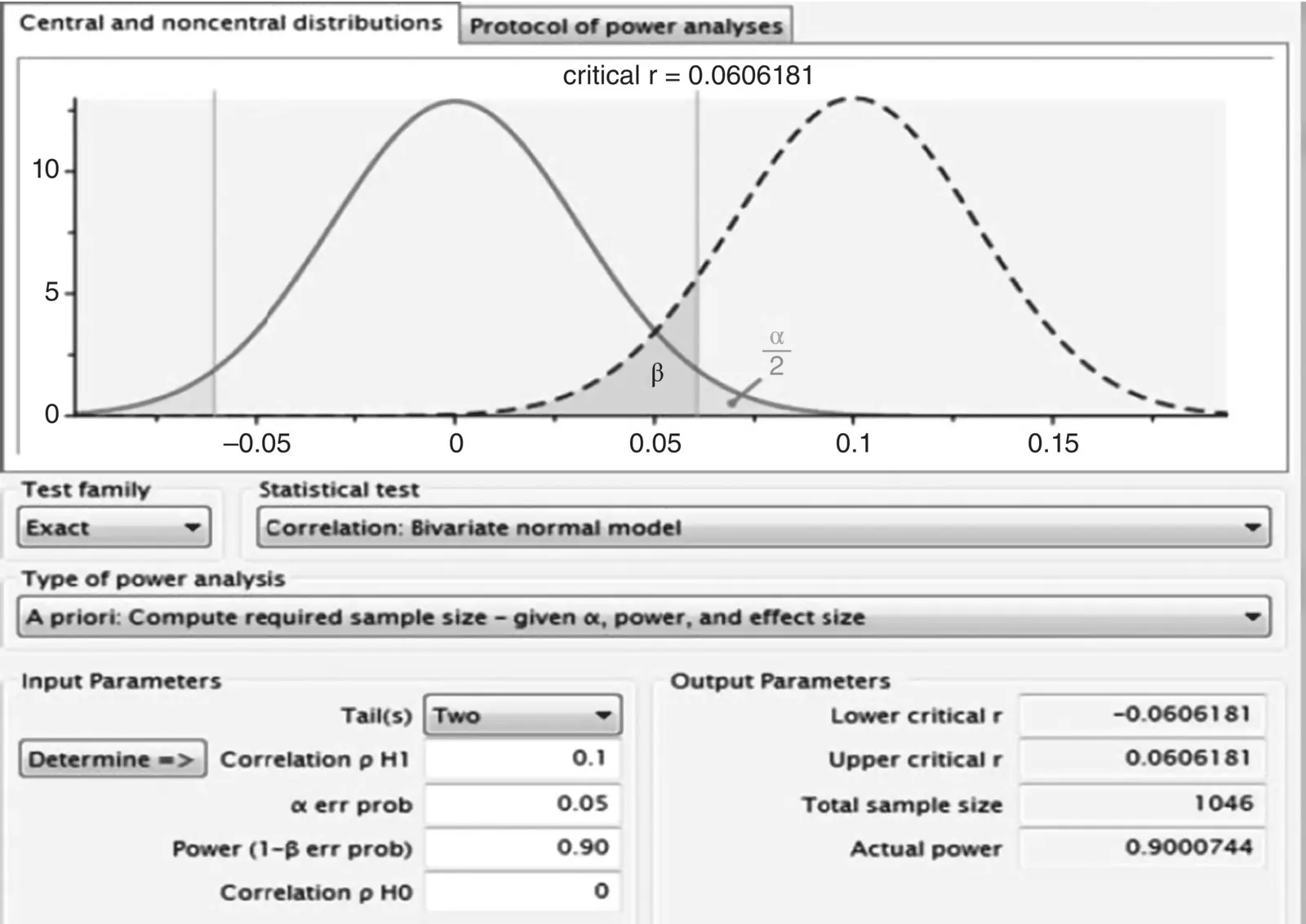
Figure 2.13G *Power output for estimating required sample size for r = 0.10.
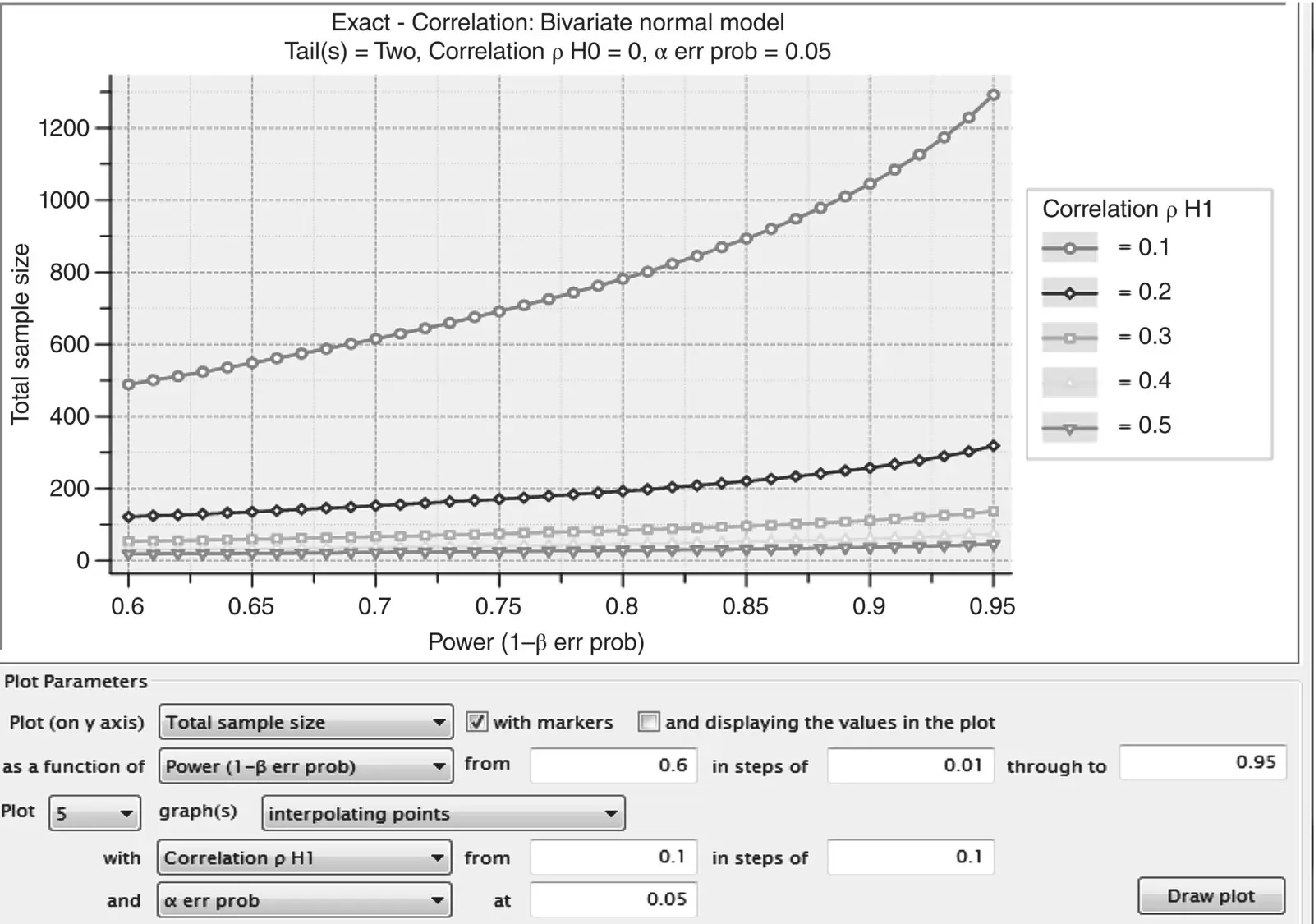
Figure 2.14Power curves generated by G *Power for detecting correlation coefficients of ρ = 0.10 to 0.50.
Especially for small hypothesized values of ρ , the required sample size for even poor to modest levels of statistical power is quite large. For example, reading off the plot in Figure 2.14, to detect ρ = 0.10, at even a relatively low power level of 0.60, one requires upward of almost 500 participants. This might explain why many studies that yield relatively small effect sizes never get published. They often have insufficient power to reject their null hypotheses. As effect size increases, required sample size drops substantially. For example, to attain a modest level of power such as 0.68 for a correlation coefficient of 0.5, one requires only 21.5 participants, as can be more clearly observed from Table 2.6which corresponds to the power curves in Figure 2.14for power ranging from 0.60 to 0.69.
Hence, one general observation from this simple power analysis for detecting ρ is that size of effect(in this case, ρ ) plays a very important role in determining estimated sample size. As a general rule, across virtually all statistical tests, if the effect you are studying is large, a much smaller sample size is required than if the effect is weak. Drawing on our analogy of the billboard sign that reads “ H 0is false,” all else equal, if the sign is in large print (i.e., strong effect), you require less “power” in your prescription glasses to detect such a large sign. If the sign is in small print (i.e., weak effect), you require much more “power” in your lenses to detect it.
2.22.1 Estimating Sample Size and Power for Independent Samples t ‐Test
For an independent‐samples t ‐test, required sample size can be estimated through R using pwr.t.test:
> pwr.t.test (n =, d =, sig.level =, power =, type = c(“two.sample”, “one.sample”, “paired”))
where, n= sample size per group, d= estimate of standardized statistical distance between means (Cohen's d), sig.level= desired significance level of the test, power= desired power level, and type= designation of the kind of t ‐test you are performing (for our example, we are performing a two‐sample test).
Table 2.6Power Estimates as a Function of Sample Size and Estimated Magnitude Under Alternative Hypothesis
| Exact – Correlation: Bivariate Normal Model Tail(s) = Two, Correlation ρ H0 = 0, α err prob = 0.05 | ||||||
|---|---|---|---|---|---|---|
| Correlation ρ H1 = 0.1 | Correlation ρ H1 = 0.2 | Correlation p HI = 0.3 | Correlation ρ HI = 0.4 | Correlation ρ HI = 0.5 | ||
| # | Power(1‐β err prob) | Total Sample Size | Total Sample Size | Total Sample Size | Total Sample Size | Total Sample Size |
| 1 | 0.600000 | 488.500 | 121.500 | 53.5000 | 29.5000 | 18.5000 |
| 2 | 0.610000 | 500.500 | 124.500 | 54.5000 | 30.5000 | 18.5000 |
| 3 | 0.620000 | 511.500 | 126.500 | 55.5000 | 30.5000 | 19.5000 |
| 4 | 0.630000 | 523.500 | 129.500 | 56.5000 | 31.5000 | 19.5000 |
| 5 | 0.640000 | 535.500 | 132.500 | 58.5000 | 32.5000 | 19.5000 |
| 6 | 0.650000 | 548.500 | 135.500 | 59.5000 | 32.5000 | 20.5000 |
| 7 | 0.660000 | 561.500 | 138.500 | 60.5000 | 33.5000 | 20.5000 |
| 8 | 0.670000 | 574.500 | 142.500 | 62.5000 | 34.5000 | 21.5000 |
| 9 | 0.680000 | 587.500 | 145.500 | 63.5000 | 34.5000 | 21.5000 |
| 10 | 0.690000 | 601.500 | 148500 | 64.5000 | 35.5000 | 22.5000 |
It would be helpful at this point to translate Cohen's d values into R 2values to learn how much variance is explained by differing d values. To convert the two, we apply the following transformation:
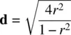
Table 2.7contains conversions for r increments of 0.10, 0.20, 0.30, etc.
To get a better feel for the relationship between Cohen's d and r 2, we obtain a plot of their values ( Figure 2.15).
As can be gleamed from Figure 2.15, the relationship between the two effect size measures is not exactly linear and increases rather sharply for rather large values (the curve is somewhat exponential).
Suppose a researcher would like to estimate required sample size for a two‐sample t ‐test, for a relatively small effect size, d = 0.41 (equal to r of 0.20), at a significance level of 0.05, with a desired power level of 0.90. We compute:
> pwr.t.test (n =, d =0.41, sig.level =.05, power =.90, type = c(“two.sample”)) Two-sample t test power calculation n = 125.9821 d = 0.41 sig.level = 0.05 power = 0.9 alternative = two.sided NOTE: n is number in *each* group
Thus, the researcher would require a sample size of approximately 126. As R emphasizes, this sample size is per group, so the totalsample size required is 126(2) = 252.
Table 2.7 Conversions for r → r2→ d. 11
| r | r 2 | d |
|---|---|---|
| 0.10 | 0.01 | 0.20 |
| 0.20 | 0.04 | 0.41 |
| 0.30 | 0.09 | 0.63 |
| 0.40 | 0.16 | 0.87 |
| 0.50 | 0.25 | 1.15 |
| 0.60 | 0.36 | 1.50 |
| 0.70 | 0.49 | 1.96 |
| 0.80 | 0.64 | 2.67 |
| 0.90 | 0.81 | 4.13 |
| 0.99 | 0.98 | 14.04 |
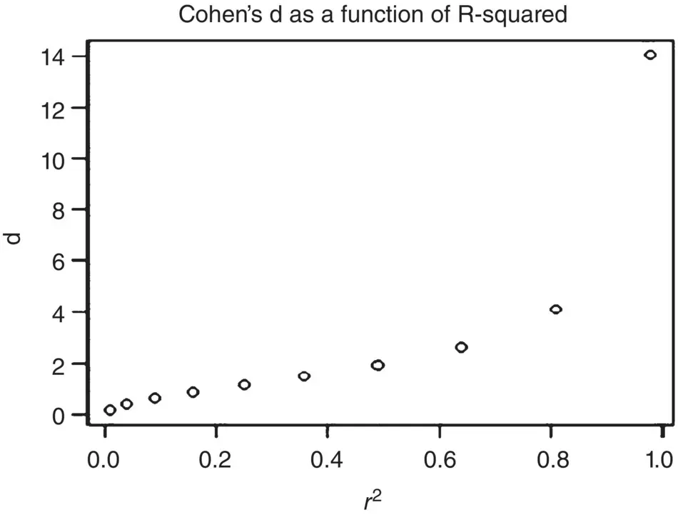
Figure 2.15Relationship between Cohen's d and R‐squared.
Читать дальшеИнтервал:
Закладка:
Похожие книги на «Applied Univariate, Bivariate, and Multivariate Statistics»
Представляем Вашему вниманию похожие книги на «Applied Univariate, Bivariate, and Multivariate Statistics» списком для выбора. Мы отобрали схожую по названию и смыслу литературу в надежде предоставить читателям больше вариантов отыскать новые, интересные, ещё непрочитанные произведения.


Обсуждение, отзывы о книге «Applied Univariate, Bivariate, and Multivariate Statistics» и просто собственные мнения читателей. Оставьте ваши комментарии, напишите, что Вы думаете о произведении, его смысле или главных героях. Укажите что конкретно понравилось, а что нет, и почему Вы так считаете.