Daniel J. Denis - Applied Univariate, Bivariate, and Multivariate Statistics

Suppose now we want to add a second response variable. Because of the generality of (2.7), this can be easily accommodated:

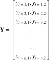
where now, a second response variable is represented in Yby a second column. That is, y i = 1, 2corresponds to individual 1 on response variable 2, y i = 2, 2is individual 2 on response variable 2, etc. We will at times refer to matrix representations throughout the book.

Performing inferential tests to help draw conclusions about population parameters is useful, but ultimately the findings of a statistical analysis should make their way into a graph or other visualization. Data visualizationis a field in itself, and with the advent of modern computing power, possibilities exist today that could only be dreamt of in the past. Simple visualizations such a histograms, boxplots, scatterplots, etc., can be useful in depicting findings but also in helping to verify assumptions that underlay the statistical model one is using. For example, since many tests of normality and equality of variances (and covariances) are relatively sensitive to the types of data to which they are applied, oftentimes researchers will generate simple plots in order to detect potential gross violations of such assumptions. We feature such techniques throughout the book.

For graphical displays meant to communicate findings (rather than test assumptions), Friendly (2000) puts the field into context:

Designing good graphics is surely an art, but as surely, it is one that ought to be informed by science… In this view, an effective graphical display, like good writing, requires an understanding of its purpose – what aspects of the data are to be communicated to the viewer. In writing, we communicate most effectively when we know our audience and tailor the message appropriately. (p. 8)

In high‐dimensional space, the challenge of graphical approaches is to summarize data into lower dimensions, while still retaining most of the information in the original data. We feature some such plots in later chapters. For a thorough account of data visualization, see datavis.ca (Friendly, 2020). For sophisticated graphics using R, consult Wickham (2009).

For now, it is useful to briefly review some basic plots for which the reader is likely already familiar.

The boxplot was a contribution of John Tukey (1977) in the spirit of what is called exploratory data analysis, or “EDA” which encouraged scientists to spend more of their energy on descriptive techniques instead of focusing exclusively on confirmatory statistical tests. Boxplots of parent heights from Galton's data appear below:

> attach(Galton) > boxplot(parent) > library(lattice) > bwplot(parent)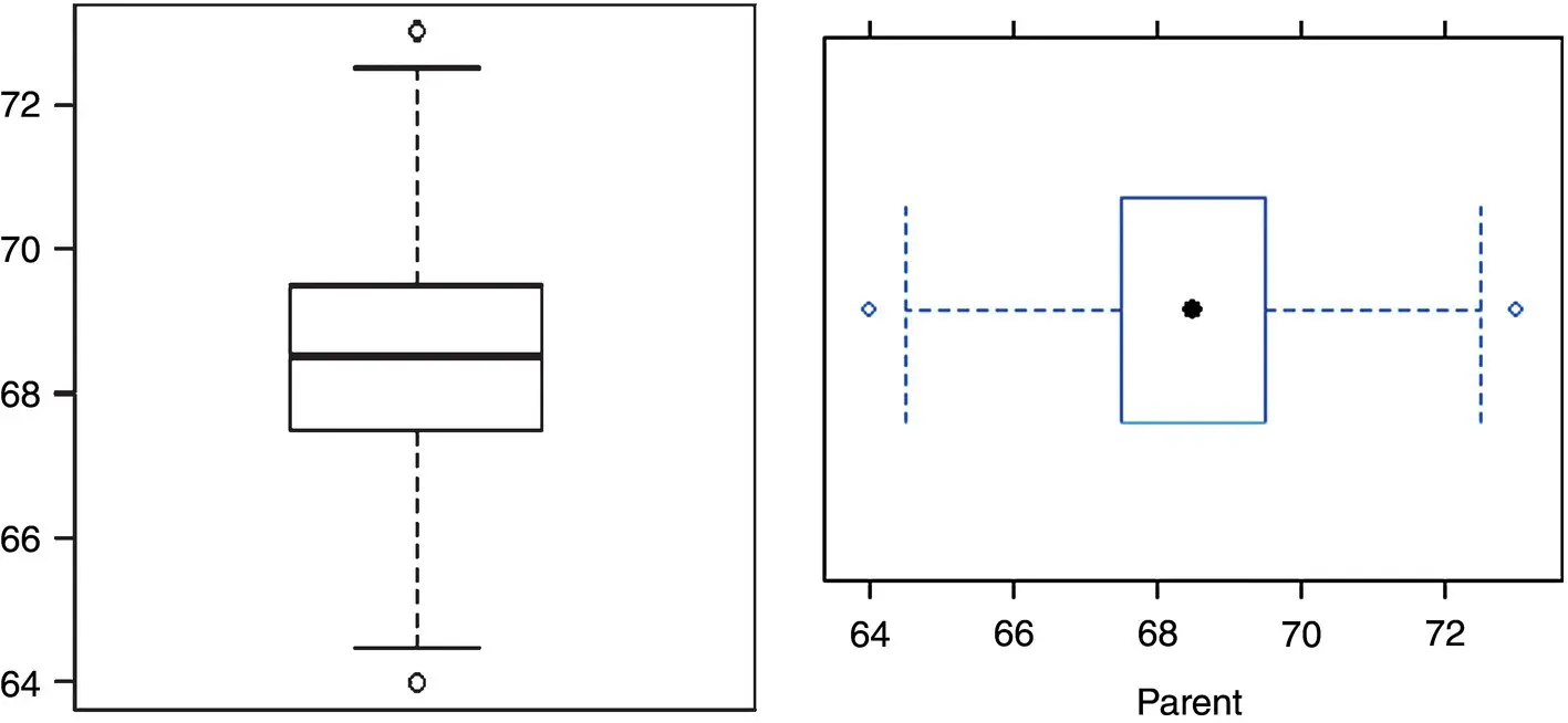

The boxplot provides what is generally known as a five‐number summaryof a distribution, of which we can obtain most of the numbers we need by the summaryfunction in R:

> summary(parent) Min. 1st Qu. Median Mean 3rd Qu. Max. 64.00 67.50 68.50 68.31 69.50 73.00

Recall that the medianis the point in the ordered data that divides the data set into two equal parts. The location of the median is computed by ( n + 1)/2. In Galton's data, there are 928 observations, and so the location of the median is at 464.5 th(i.e., (928 + 1)/2) point in the ordered data set. For parent, this value is equal to 68.50. The first and third quartiles represent the 25th and 75th percentiles and are 67.50 and 69.50 respectively. We can also compute the range as

> range(parent) [1] 64 73

We can also generate boxplots by category. Throughout the book, we use Fisher's iris data (Fisher, 1936) in which flower characteristics such as sepal and petal length are categorized by species of flower. We plot sepal length by species:

> library(lattice) > attach(iris) > bwplot(Sepal.Length ~ Species)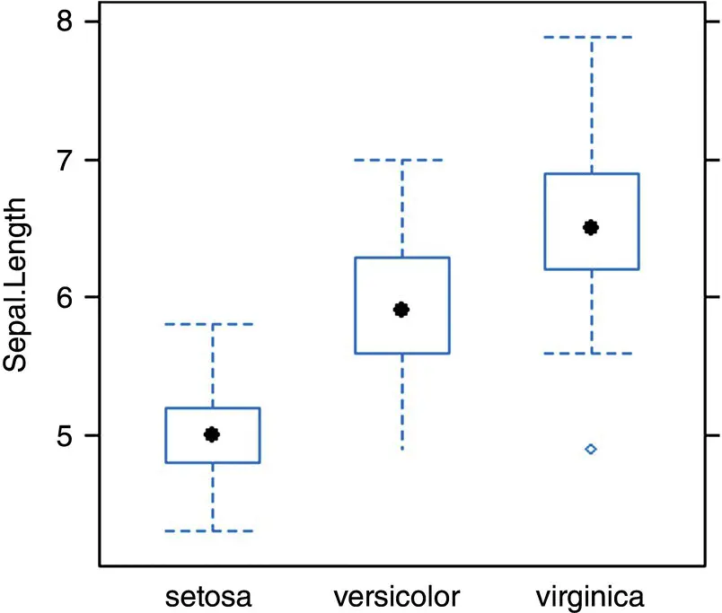

Data points falling beyond the whiskers of the plots may reveal the presence of outliers, and should be investigated (though of course, not necessarily deleted, see Section for a discussion). If you are completely unfamiliar with boxplots, see Denis (2020) for an overview.

Stem‐and‐leaf plotsare also easily produced. These visual displays are kind of “naked histograms,” because they reveal the actual observations in the data while also providing information about their frequency of occurrence. In 1710, John Arbuthnot analyzed data on the ratios of males to female births in London from 1629 to 1710 and in so doing made an argument for these births being a function of a “divine being” (Arbuthnot, 1710; Shoesmith, 1987). One of his variables was the number of male christenings (i.e., baptisms) over the period 1629–1710. We generate a stem‐and‐leaf plot in R of these male christenings using package aplpack(Wolf and Bielefeld, 2014), for which the “leaves” are corresponding hundreds. For example, in the following plot, the first value of 2|8 would appear to represent a value of 2800 but is rounded down from the actual value in the data (which is also the minimum) of 2890. The maximum in the data is actually equal to 8426, but is represented by 8400 (i.e., 8|0012334):

> install.packages(“aplpack”) > library(aplpack) > library(HistData) > attach(Arbuthnot) > stem.leaf(Males) 1 | 2: represents 1200 leaf unit: 100 n: 82 1 2. | 8 10 3* | 011222334 15 3. | 66777 18 4* | 014 25 4. | 6777899 36 5* | 01112233444 38 5. | 56 (11) 6* | 00001122444 33 6. | 5555899 26 7* | 244 23 7. | 5555666666778999 7 8* | 0012334

The workhorse for establishing statistical evidence in the social and natural sciences is the method of null hypothesis significance testing(or, “NHST” for short). However, since its inception with R.A. Fisher in the early 1900s, the significance test has been the topic of much debate, both statistical and philosophical. Throughout much of this book, NHST is regularly used to evaluate null hypotheses in methods such as the analysis of variance, regression, and various multivariate procedures. Indeed, the procedure is universally used in most statistical methods.

It behooves us then, before embarking on all of these methodologies, to discuss the nature of the null hypothesis significance test, and clearly demonstrate what it actually means, not only in a statistical context but also in how it should be interpreted in a researchor substantivecontext.

The purpose of this final section of the present chapter is to provide a clear and concise demonstration and summary of the factors that influence the size of a computed p ‐value in virtually every statistical significance test. Understanding why statements such as “ p < 0.05” can be reflective of even the smallest and trivial of effects is critical for the practitioner or researcher to appreciate if he or she is to assess and appraise statistical evidence in an intelligent and thoughtful manner. It is not an exaggeration to say that if one does not understand the make‐up of a p‐value and the factors that directly influence its size, one cannot properly evaluate statistical evidence, nor should one even make the attempt to do so. Though these arguments are not new and have been put forth by even the very best of methodologists (e.g., see Cohen, 1990; Meehl, 1978) there is evidence to suggest that many practitioners and researchers do not understand the factors that determine the size of a p ‐value (Gigerenzer, 2004). To emphasize once again—understanding the determinants of a p ‐value and what makes p ‐values distinct from effect sizes is not simply “fashionable.” Rather, it is absolutely mandatory for any attempt to properly evaluate statistical evidence in a research report. Does the paper you're reading provide evidence of a successful treatment for cancer? If you do not understand the distinctions between p‐values and effect sizes, you will be unable to properly assess the evidence. It is that important. As we will see, stating a result as “statistically significant” does not in itself tell you whether the treatment works or does not work, and in some cases, tells you very little at all from a scientific vantage point.