Daniel J. Denis - Applied Univariate, Bivariate, and Multivariate Statistics

The resulting value for z Mis quite large at 10. Consider now what happens if we increase σ from 2 to 10:

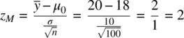
Notice that the value of z Mhas decreased from 10 to 2. Consider now what happens if we increase σ even more to a value of 20 as we had originally:

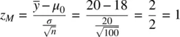
When σ = 20, the value of z Mis now equal to 1, which is no longer statistically significant at p < 0.05. Be sure to note that the distance between means has remained constant. In other words, and this is important, z M did not decrease in magnitude by altering the actual distance between the sample mean and the population mean, but rather decreased in magnitude only by a change in σ .

What this means is that given a constant distance between means , whether or not z Mwill or will not be statistically significant can be manipulated by changing the value of σ . Of course, a researcher would never arbitrarily manipulate σ directly. The way to decrease σ would be to sample from a population with less variability. The point is that decisions regarding whether a “positive” result occurred in an experiment or study should not be solely a function of whether one is sampling from a population with small or large variance!

Suppose now we again assume the distance between means to be equal to 2. We again set the value of σ at 2. With these values set and assumed constant, consider what happens to z Mas we increase the sample size n from 16 to 49 to 100. We first compute z Massuming a sample size of 16:

With a sample size of 16, the computed value for z Mis equal to 4. When we increase the sample size to 49, again, keeping the distance between means constant, as well as the population standard deviation constant, we obtain:

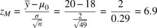
We see that the value of z Mhas increased from 4 to 6.9 as a result of the larger sample size. If we increase the sample size further, to 100, we get

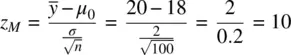
and see that as a result of the even larger sample size, the value of z Mhas increased once again, this time to 10. Again, we need to emphasize that the observed increase in z Mis occurring not as a result of changing values for or σ , as these values remained constant in our above computations. Rather, the magnitude of z M increased as a direct result of an increase in sample size, n , alone. In many research studies, the achievement of a statistically significant result may simply be indicative that the researcher gathered a minimally sufficient sample size that resulted in z M falling in the tail of the z distribution. In other cases, the failure to reject the null may in reality simply indicate that the investigator had insufficient sample size. The point is that unless one knows how n can directly increase or decrease the size of a p ‐value, one cannot be in a position to understand, in a scientific sense, what the p ‐value actually means, or intelligently evaluate the statistical evidence before them.

The simplicity of these demonstrations is surpassed only by their profoundness. In our simple example of the one‐sample z ‐test for a mean, we have demonstrated that the size of z Mis a direct function of three elements: (1) distance , (2) population standard deviation σ , and (3) sample size n . A change in anyof these while holding the others constant will necessarily, through nothing more than the consequences of how the significance test is constructed and functionally defined, result in a change in the size of z M. The implication of this is that one can make z Mas small or as large as one would like by choosing to do a study or experiment such that the combination of , σ , and n results in a z Mvalue that meets or exceeds a pre‐selected criteria of statistical significance.

The important point here is that a large value of z Mdoes not necessarily mean something of any practicalor scientificsignificance occurred in the given study or experiment. This fact has been reiterated countless times by the best of methodologists, yet too often researchers fail to emphasize this extremely important truth when discussing findings:

A p‐value, no matter how small or large, does not necessarily equate to the success or failure of a given experiment or study.

Too often a statement of “ p < 0.05” is recited to an audience with the implication that somehow this necessarily constitutes a “scientific finding” of sorts. This is entirely misleading, and the practice needs to be avoided. The solution, as we will soon discuss, is to pair the p ‐value with a report of the effect size.

To demonstrate how adjusting the inputs to z Mcan have a direct impact on the obtained p ‐value, consider the situation in which a school psychologist practitioner hypothesizes that as a result of an intensified program implementation in her school, she believes that her school's students, on average, will have a higher achievement mean compared to the national average of students in the same grade. Suppose that the national average on a given standardized performance test is equal to 100. If the school psychologist is correct that her students are, on average, more advanced performance‐wise than the national average, then her students should, on average, score higher than the national mark of 100. She decides to sample 100 students from her school and obtains a sample achievement mean of . Thus, the distance between means is equal to 101 – 100 = 1. She computes the estimated population standard deviation s equal to 10. Because she is estimating σ 2with s 2, she computes a one‐sample t ‐test rather than a z ‐test. Her computation of the ensuing t is: