Daniel J. Denis - Applied Univariate, Bivariate, and Multivariate Statistics
Здесь есть возможность читать онлайн «Daniel J. Denis - Applied Univariate, Bivariate, and Multivariate Statistics» — ознакомительный отрывок электронной книги совершенно бесплатно, а после прочтения отрывка купить полную версию. В некоторых случаях можно слушать аудио, скачать через торрент в формате fb2 и присутствует краткое содержание. Жанр: unrecognised, на английском языке. Описание произведения, (предисловие) а так же отзывы посетителей доступны на портале библиотеки ЛибКат.
- Название:Applied Univariate, Bivariate, and Multivariate Statistics
- Автор:
- Жанр:
- Год:неизвестен
- ISBN:нет данных
- Рейтинг книги:5 / 5. Голосов: 1
-
Избранное:Добавить в избранное
- Отзывы:
-
Ваша оценка:
Applied Univariate, Bivariate, and Multivariate Statistics: краткое содержание, описание и аннотация
Предлагаем к чтению аннотацию, описание, краткое содержание или предисловие (зависит от того, что написал сам автор книги «Applied Univariate, Bivariate, and Multivariate Statistics»). Если вы не нашли необходимую информацию о книге — напишите в комментариях, мы постараемся отыскать её.
contains an accessible introduction to statistical modeling techniques commonly used in the social and behavioral sciences. The text offers a blend of statistical theory and methodology and reviews both the technical and theoretical aspects of good data analysis.
Featuring applied resources at various levels, the book includes statistical techniques using software packages such as R and SPSS®. To promote a more in-depth interpretation of statistical techniques across the sciences, the book surveys some of the technical arguments underlying formulas and equations. The thoroughly updated edition includes new chapters on nonparametric statistics and multidimensional scaling, and expanded coverage of time series models. The second edition has been designed to be more approachable by minimizing theoretical or technical jargon and maximizing conceptual understanding with easy-to-apply software examples. This important text:
Offers demonstrations of statistical techniques using software packages such as R and SPSS® Contains examples of hypothetical and real data with statistical analyses Provides historical and philosophical insights into many of the techniques used in modern social science Includes a companion website that includes further instructional details, additional data sets, solutions to selected exercises, and multiple programming options Written for students of social and applied sciences,
offers a text to statistical modeling techniques used in social and behavioral sciences.
Applied Univariate, Bivariate, and Multivariate Statistics — читать онлайн ознакомительный отрывок
Ниже представлен текст книги, разбитый по страницам. Система сохранения места последней прочитанной страницы, позволяет с удобством читать онлайн бесплатно книгу «Applied Univariate, Bivariate, and Multivariate Statistics», без необходимости каждый раз заново искать на чём Вы остановились. Поставьте закладку, и сможете в любой момент перейти на страницу, на которой закончили чтение.
Интервал:
Закладка:
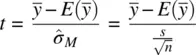
was found to be distributed as a t statistic on n − 1 degrees of freedom. Again, the t distribution is most useful for when sample sizes are rather small. For larger samples, as mentioned, the t distribution converges to that of the z distribution. If you are using rather large samples, say approximately 100 or more, whether you evaluate your null hypothesis using a z or t distribution will not matter much, because the critical values for z and t for such degrees of freedom (99 for the one‐sample case) will be relatively alike, that practically at least, the two test statistics can be considered more or less equal. For even larger samples, the convergence is that much more fine‐tuned.
The concept of convergence between z and t can be easily illustrated by inspecting the variance of the t distribution. Unlike the z distribution where the variance is set at 1.0 as a constant, the variance of the t distribution is defined as:

where v are the degrees of freedom. For small degrees of freedom, such as v = 5, the variance of the t distribution is equal to:
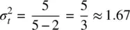
Note what happens as v increases, the ratio  gets closer and closer to 1.0, which is the precise variance of the z distribution. For example, v = 20 yields:

which is already quite close to the variance of a standardized normal variable z (i.e., 1.0). Hence, we can say more formally
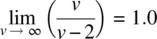
That is, as v increases without bound, the variance of the t distribution equals that of the z distribution, which is equal to 1.0.
We demonstrate the use of the one‐sample t ‐test using SPSS. Consider the following small, hypothetical data on IQ scores on five individuals:
IQ 105 98 110 105 95
Suppose that the hypothesized mean IQ in the population is equal to 100. The question we want to ask is— Is it reasonable to assume that our sampled data could have arisen from a population with mean IQ equal to 100?We assume we have no knowledge of the population standard deviation, and hence must estimate it from our sample data. To perform the one‐sample t ‐test in SPSS, we compute:
T-TEST /TESTVAL=100 /MISSING=ANALYSIS /VARIABLES=IQ /CRITERIA=CI(.95).
The line /TESTVAL = 100inputs the test value for our hypothesis test, which for our null hypothesis is equal to 100. We have also requested a 95% confidence interval for the mean difference.
| One‐Sample Statistics | ||||
| N | Mean | SD | SE Mean | |
| IQ | 5 | 102.6000 | 6.02495 | 2.69444 |
We confirm from the above that the size of our sample is equal to 5, and the mean IQ for our sample is equal to 102.60 with standard deviation 6.02. The standard error of the mean reported by SPSS of 2.69 is actually not the truestandard error of the mean. It is the estimatedstandard error of the mean, since recall that we did not have knowledge of the population variance (otherwise we would have been performing a z ‐test instead of a t ‐test).
| One‐Sample Test | ||||||
|---|---|---|---|---|---|---|
| Test Value = 100 | ||||||
| 95% Confidence Interval of the Difference | ||||||
| t | Df | Sig. (2‐tailed) | Mean Difference | Lower | Upper | |
| IQ | 0.965 | 4 | 0.389 | 2.60000 | −4.8810 | 10.0810 |
We note from the above output:
Our obtained t‐statistic is equal to 0.965 and is evaluated on four degrees of freedom (i.e., n − 1 = 5 − 1 = 4). We lose a degree of freedom because recall that in estimating the population variance σ2 with s2, we had to compute a sample mean and hence this value is regarded as “fixed” as we carry on with our t‐test. Hence, we lose a single degree of freedom.
The two‐tailed p‐value is equal to 0.389, which, assuming we had set our criteria for rejection at α = 0.05, leads us to the decision to not reject the null hypothesis. The two‐tailed (as opposed to one‐tailed or directional) nature of the statistical test in this example means that we allow for a rejection of the null hypothesis in either direction from the value stated under the null. Since our null hypothesis is μ0 = 100, it means we were prepared to reject the null hypothesis for observed values of the sample mean that deviate “significantly” either greater than or less than 100. Since our significance level was set at 0.05, this means that we have 0.05/2 = 0.025 area in each end of the t distribution to specify as our rejection region for the test. The question we are asking of our sample mean is—What is the probability of observing a sample mean that falls much greater OR much less than 100? Because the observed sample mean can only fall in one tail or the other on any single trial (i.e., we are conducting a single “trial” when we run this experiment a single time), this implies these two events are mutually exclusive, which by the addition rule for mutually exclusive events, we can add them. When we add their probabilities, we get 0.025 + 0.025 = 0.05, which, of course, is our significance level for the test.
The actual mean difference observed is equal to 2.60, which was computed by taking the mean of our sample, that of 102.6 and subtracting the mean hypothesized under the null hypothesis, that of 100 (i.e., 102.6 – 100 = 2.60).
The 95% confidence interval of the difference is interpreted to mean that with 95% confidence, the interval with lower bound −4.8810 and upper bound 10.0810 will capture the true parameter, which in this case is the population mean difference. We can see that 0 lies within the limits of the confidence interval, which again confirms why we were unable to reject the null hypothesis at the 0.05 level of significance. Had zero lay outside of the confidence interval limits, this would have been grounds to reject the null at a significance level of 0.05 (and consequently, we would have also obtained a p‐value of less than 0.05 for our significance test). Recall that the true mean (i.e., parameter) is not the random component. Rather, the sample is the random component, on which the interval is then computed. It is important to emphasize this distinction when interpreting the confidence interval.
We can easily generate the same t ‐test in R. We first generate the vector of data then carry on with the one‐sample t ‐test, which we notice mirrors the findings obtained in SPSS:
Читать дальшеИнтервал:
Закладка:
Похожие книги на «Applied Univariate, Bivariate, and Multivariate Statistics»
Представляем Вашему вниманию похожие книги на «Applied Univariate, Bivariate, and Multivariate Statistics» списком для выбора. Мы отобрали схожую по названию и смыслу литературу в надежде предоставить читателям больше вариантов отыскать новые, интересные, ещё непрочитанные произведения.


Обсуждение, отзывы о книге «Applied Univariate, Bivariate, and Multivariate Statistics» и просто собственные мнения читателей. Оставьте ваши комментарии, напишите, что Вы думаете о произведении, его смысле или главных героях. Укажите что конкретно понравилось, а что нет, и почему Вы так считаете.