Daniel J. Denis - Applied Univariate, Bivariate, and Multivariate Statistics
Здесь есть возможность читать онлайн «Daniel J. Denis - Applied Univariate, Bivariate, and Multivariate Statistics» — ознакомительный отрывок электронной книги совершенно бесплатно, а после прочтения отрывка купить полную версию. В некоторых случаях можно слушать аудио, скачать через торрент в формате fb2 и присутствует краткое содержание. Жанр: unrecognised, на английском языке. Описание произведения, (предисловие) а так же отзывы посетителей доступны на портале библиотеки ЛибКат.
- Название:Applied Univariate, Bivariate, and Multivariate Statistics
- Автор:
- Жанр:
- Год:неизвестен
- ISBN:нет данных
- Рейтинг книги:5 / 5. Голосов: 1
-
Избранное:Добавить в избранное
- Отзывы:
-
Ваша оценка:
Applied Univariate, Bivariate, and Multivariate Statistics: краткое содержание, описание и аннотация
Предлагаем к чтению аннотацию, описание, краткое содержание или предисловие (зависит от того, что написал сам автор книги «Applied Univariate, Bivariate, and Multivariate Statistics»). Если вы не нашли необходимую информацию о книге — напишите в комментариях, мы постараемся отыскать её.
contains an accessible introduction to statistical modeling techniques commonly used in the social and behavioral sciences. The text offers a blend of statistical theory and methodology and reviews both the technical and theoretical aspects of good data analysis.
Featuring applied resources at various levels, the book includes statistical techniques using software packages such as R and SPSS®. To promote a more in-depth interpretation of statistical techniques across the sciences, the book surveys some of the technical arguments underlying formulas and equations. The thoroughly updated edition includes new chapters on nonparametric statistics and multidimensional scaling, and expanded coverage of time series models. The second edition has been designed to be more approachable by minimizing theoretical or technical jargon and maximizing conceptual understanding with easy-to-apply software examples. This important text:
Offers demonstrations of statistical techniques using software packages such as R and SPSS® Contains examples of hypothetical and real data with statistical analyses Provides historical and philosophical insights into many of the techniques used in modern social science Includes a companion website that includes further instructional details, additional data sets, solutions to selected exercises, and multiple programming options Written for students of social and applied sciences,
offers a text to statistical modeling techniques used in social and behavioral sciences.
Applied Univariate, Bivariate, and Multivariate Statistics — читать онлайн ознакомительный отрывок
Ниже представлен текст книги, разбитый по страницам. Система сохранения места последней прочитанной страницы, позволяет с удобством читать онлайн бесплатно книгу «Applied Univariate, Bivariate, and Multivariate Statistics», без необходимости каждый раз заново искать на чём Вы остановились. Поставьте закладку, и сможете в любой момент перейти на страницу, на которой закончили чтение.
Интервал:
Закладка:
We see that r sof 0.425 is slightly less than was Pearson r of 0.459.
To understand why Spearman's rank correlation and Pearson coefficient differ, consider data ( Table 2.5) on the rankings of favorite movies for two individuals. In parentheses are subjective scores of “favorability” of these movies, scaled 1–10, where 1 = least favorable and 10 = most favorable.
From the table, we can see that Bill very much favors Star Wars (rating of 10) while least likes Batman (rating of 2.1). Mary's favorite movie is Scarface (rating of 9.7) while her least favorite movie is Batman (rating of 7.6). We will refer to these subjective scores in a moment. For now, we focus only on the ranks. For instance, Bill's ranking of Scarface is third, while Mary's ranking of Star Wars is third.
Table 2.5 Favorability of Movies for Two Individuals in Terms of Ranks
| Movie | Bill | Mary |
|---|---|---|
| Batman | 5 (2.1) | 5 (7.6) |
| Star Wars | 1 (10.0) | 3 (9.0) |
| Scarface | 3 (8.4) | 1 (9.7) |
| Back to the Future | 4 (7.6) | 4 (8.5) |
| Halloween | 2 (9.5) | 2 (9.6) |
Actual scores on the favorability measure are in parentheses.
To compute Spearman's r sin R the “long way,” we generate two vectors that contain the respective rankings:
> bill <- c(5, 1, 3, 4, 2) > mary <- c(5, 3, 1, 4, 2)
Because the data are already in the form of ranks, both Pearson r and Spearman rho will agree:
> cor(bill, mary) [1] 0.6 > cor(bill, mary, method = “spearman”) > 0.6
Note that by default, R returns the Pearson correlation coefficient. One has to specify method = “spearman”to get r s. Consider now what happens when we correlate, instead of rankings, the actual subjective favorability scores corresponding to the respective ranks. When we plot the favorability data, we obtain:
> bill.sub <- c(2.1, 7.6, 8.4, 9.5, 10.0) > mary.sub <- c(7.6, 8.5, 9.0, 9.6, 9.7) > plot(mary.sub, bill.sub) 
Note that though the relationship is not perfectly linear, each increase in Bill's subjective score is nonetheless associated with an increase in Mary's subjective score. When we compute Pearson's r on this data, we obtain:
> cor(bill.sub, mary.sub) [1] 0.9551578
However, when we compute r s, we get:
> cor(bill.sub, mary.sub, method = "spearman") [1] 1
Spearman's r sis equal to 1.0 because the rankings of movie preferences are perfectly monotonically increasing(i.e., for each increase in movie preference along the abscissa corresponds an increase in movie preference along the ordinate). In the case of Pearson's, the correlation is less than 1.0 because r captures the linearrelationship among variables and not simply a monotonically increasing one. Hence, a high magnitude coefficient for Spearman's essentially tells us that two variables are “moving together,” but it does not necessarily imply the relationship is a linear one. A similar test that measures rank correlation is that of Kendall's rank‐order correlation. See Siegel and Castellan (1988, p. 245) for details.
2.20 STUDENT'S t DISTRIBUTION
The density for Student's t is given by (Shao, 2003):
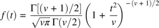
where Γ is the gamma function and v are degrees of freedom. For small degrees of freedom v , the t distribution is quite distinct from the standard normal. However, as degrees of freedom increase, the t distribution converges to that of a normal density ( Figure 2.11). That is, in the limit, f ( t ) → f ( z ), or a bit more formally, 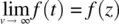 .
.
The fact that t converges to z for large degrees of freedom but is quite distinct from z for small degrees of freedom is one reason why t distributions are often used for small sampleproblems. When sample size is large, and so consequently are degrees of freedom, whether one treats a random variable as t or z will make little difference in terms of computed p ‐values and decisions on respective null hypotheses. This is a direct consequence of the convergence of the two distributions for large degrees of freedom. For a historical overview of how t ‐distributions came to be, consult Zabell (2008).
2.20.1 t ‐Tests for One Sample
When we perform hypothesis testing using the z distribution, we assume we have knowledge of the population variance σ 2. Having direct knowledge of σ 2is the most idealand preferable of circumstances. When we know σ 2, we can compute the standard error of the mean directly as

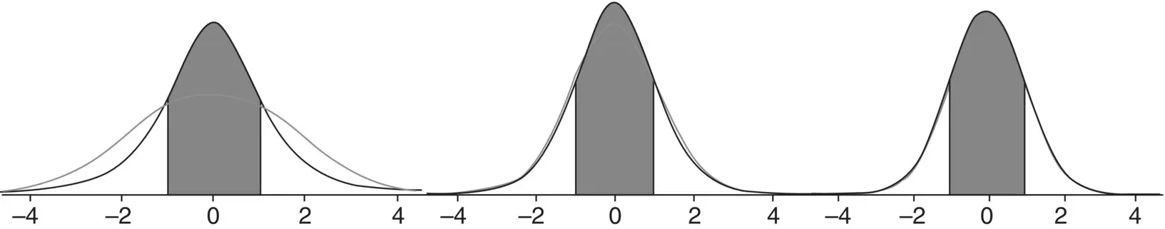
Figure 2.11Student's t versus normal densities for 3 (left), 10 (middle), and 50 (right) degrees of freedom. As degrees of freedom increase, the limiting form of the t distribution is the z distribution.
Recall that the form of the one‐sample z test for the mean is given by

where the numerator  represents the distance between the sample mean and the population mean μ 0under the null hypothesis, and the denominator
  is the standard error of the mean.
In most research contexts, from simple to complex, we usually do not have direct knowledge of σ 2. When we do not have knowledge of it, we use the next best thing, an estimate of it. We can obtain an unbiased estimate of σ 2by computing s 2on our sample. When we do so, however, and use s 2in place of σ 2, we can no longer pretend to “know” the standard error of the mean. Rather, we must concede that all we are able to do is estimate it. Our estimate of the standard error of the mean is thus given by:

When we use s 2(where  ) in place of σ 2, our resulting statistic is no longer a z statistic. That is, we say the ensuing statistic is no longer distributedas a standard normal variable (i.e., z ). If it is not distributed as z , then what is it distributed as? Thanks to William Sealy Gosset who in 1908 worked for Guinness Breweriesunder the pseudonym “Student” (Zabell, 2008), the ratio
Интервал:
Закладка:
Похожие книги на «Applied Univariate, Bivariate, and Multivariate Statistics»
Представляем Вашему вниманию похожие книги на «Applied Univariate, Bivariate, and Multivariate Statistics» списком для выбора. Мы отобрали схожую по названию и смыслу литературу в надежде предоставить читателям больше вариантов отыскать новые, интересные, ещё непрочитанные произведения.


Обсуждение, отзывы о книге «Applied Univariate, Bivariate, and Multivariate Statistics» и просто собственные мнения читателей. Оставьте ваши комментарии, напишите, что Вы думаете о произведении, его смысле или главных героях. Укажите что конкретно понравилось, а что нет, и почему Вы так считаете.