Daniel J. Denis - Applied Univariate, Bivariate, and Multivariate Statistics
Здесь есть возможность читать онлайн «Daniel J. Denis - Applied Univariate, Bivariate, and Multivariate Statistics» — ознакомительный отрывок электронной книги совершенно бесплатно, а после прочтения отрывка купить полную версию. В некоторых случаях можно слушать аудио, скачать через торрент в формате fb2 и присутствует краткое содержание. Жанр: unrecognised, на английском языке. Описание произведения, (предисловие) а так же отзывы посетителей доступны на портале библиотеки ЛибКат.
- Название:Applied Univariate, Bivariate, and Multivariate Statistics
- Автор:
- Жанр:
- Год:неизвестен
- ISBN:нет данных
- Рейтинг книги:5 / 5. Голосов: 1
-
Избранное:Добавить в избранное
- Отзывы:
-
Ваша оценка:
Applied Univariate, Bivariate, and Multivariate Statistics: краткое содержание, описание и аннотация
Предлагаем к чтению аннотацию, описание, краткое содержание или предисловие (зависит от того, что написал сам автор книги «Applied Univariate, Bivariate, and Multivariate Statistics»). Если вы не нашли необходимую информацию о книге — напишите в комментариях, мы постараемся отыскать её.
contains an accessible introduction to statistical modeling techniques commonly used in the social and behavioral sciences. The text offers a blend of statistical theory and methodology and reviews both the technical and theoretical aspects of good data analysis.
Featuring applied resources at various levels, the book includes statistical techniques using software packages such as R and SPSS®. To promote a more in-depth interpretation of statistical techniques across the sciences, the book surveys some of the technical arguments underlying formulas and equations. The thoroughly updated edition includes new chapters on nonparametric statistics and multidimensional scaling, and expanded coverage of time series models. The second edition has been designed to be more approachable by minimizing theoretical or technical jargon and maximizing conceptual understanding with easy-to-apply software examples. This important text:
Offers demonstrations of statistical techniques using software packages such as R and SPSS® Contains examples of hypothetical and real data with statistical analyses Provides historical and philosophical insights into many of the techniques used in modern social science Includes a companion website that includes further instructional details, additional data sets, solutions to selected exercises, and multiple programming options Written for students of social and applied sciences,
offers a text to statistical modeling techniques used in social and behavioral sciences.
Applied Univariate, Bivariate, and Multivariate Statistics — читать онлайн ознакомительный отрывок
Ниже представлен текст книги, разбитый по страницам. Система сохранения места последней прочитанной страницы, позволяет с удобством читать онлайн бесплатно книгу «Applied Univariate, Bivariate, and Multivariate Statistics», без необходимости каждый раз заново искать на чём Вы остановились. Поставьте закладку, и сможете в любой момент перейти на страницу, на которой закончили чтение.
Интервал:
Закладка:
> library(ggplot2) > qplot(child, parent, data = Galton, geom = c("point", "smooth")) 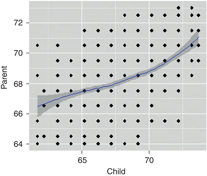
One drawback of such a simple plot is that the frequency of data points in the bivariate space cannot be known by inspection of the plot alone. Jitteringis a technique that allows one to visualize the density of points at each parent–child pairing. By jittering, we can see where most of the data fall in the parent–child scatterplot (i.e., points are concentrated toward the center of the plot):
> qplot(child, parent, geom = "jitter") 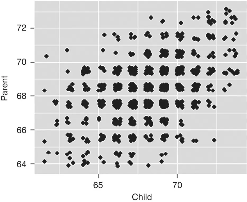
2.17 PSYCHOMETRIC VALIDITY, RELIABILITY: A COMMON USE OF CORRELATION COEFFICIENTS
Correlation coefficients, specifically the Pearson correlation, are employed in virtually all fields of study, and without the invention or discovery of correlation, most modern‐day statistics would simply not exist. This is especially true for the field of psychometrics, which is the science that deals with the measurement of psychological qualities such as intelligence, self‐esteem, motivation, among others. Psychometrics features the development of psychometric tests purported to measure the construct of interest. For an excellent general introduction to psychometrics, consult McDonald (1999).
When developing psychometric instruments, two statistical characteristics of these tests are especially important: (1) validity, and (2) reliability. Validity of a test takes many forms, including face validity, criterion validity, and most notably, construct validity. Construct validity attempts to assess whether a purported psychometric test actually measures what it was designed to measure, and one way of evaluating construct validity is to correlate the newly developed measure with that of an existing measure that is already known to successfully measure the construct.
For example, in the area of depression assessment, the Beck Depression Inventory (BDI)is a popular self‐report measure often used in evaluating one's level or symptoms of depression. Now, if we were to develop a new test, in order to learn whether that new test measures something called “depression,” we may wish to compute a Pearson correlation of that measure with the BDI. To the extent that the correlation is relatively high, we might tentatively conclude that the new measure is assessing the same (or at least a similar) construct as that of the BDI. Not surprisingly, these correlations in this context often go by the name of validitiesin the psychometric literature. If a test lacks construct validity, then there is little guarantee that it is measuring the construct under investigation. Fields such as psychology depend on such construct validation to gain some sense of certainty that their measures are tapping into what they are most interested in. Clinical psychology, especially, depends on the strength of such things as construct validity to secure a sense of sureness that their diagnostic tests are measuring what they are thought to measure. Without psychometrics, clinical testing in this way would be no more advanced than folk or “pop” psychology tests we often find on the internet, which are usually wholly unscientific.
The second area of concern, that of reliability, is just as important. Two popular and commonly used forms of reliability in psychometrics are those of test–retest and internal consistency reliability. Test–retestreliability evaluates the consistency of test scores across one or more measurement time points. For example, if I measured your IQ today, and the test was worth its salt, I should expect that a measurement of your IQ a month from now should, within a reasonable margin of error, generate a similar score, assuming it was administered under standardized conditions both times. If not, we might doubt the test's reliability. The Pearson correlation coefficient is commonly used to evaluate test–retest reliability, where a higher‐than‐not coefficient between testings is desirable. In addition to test–retest, we often would like a measure of what is known as the internal consistencyof a measure, which, though having potentially several competing meanings (e.g., see Tang et al., 2014), can be considered to assess how well items on a scale “hang together,” which is informal language for whether or not items on a test are interrelated(Schmitt, 1996). For this assessment, we can compute Cronbach's alpha, which we will now briefly demonstrate in SPSS.
As a very small‐scale example, suppose we have a test having only five items (items 1 through 5 in the SPSS data view), and would like to assess the internal consistency of the measure using Cronbach's alpha. Suppose the scores on the items are as follows:
| Item_1 | Item_2 | Item_3 | Item_4 | Item_5 | |
| 1 | 10.00 | 12.00 | 15.00 | 11.00 | 12.00 |
| 2 | 12.00 | 18.00 | 12.00 | 12.00 | 1.00 |
| 3 | 8.00 | 16.00 | 14.00 | 14.00 | 4.00 |
| 4 | 6.00 | 8.00 | 16.00 | 8.00 | 6.00 |
| 5 | 4.00 | 7.00 | 8.00 | 7.00 | 5.00 |
| 6 | 6.00 | 6.00 | 3.00 | 7.00 | 3.00 |
| 7 | 3.00 | 4.00 | 6.00 | 5.00 | 8.00 |
| 8 | 7.00 | 3.00 | 7.00 | 9.00 | 9.00 |
| 9 | 8.00 | 9.00 | 4.00 | 10.00 | 10.00 |
| 10 | 9.00 | 5.00 | 6.00 | 11.00 | 12.00 |
To compute a Cronbach's alpha, and obtain a handful of statistics useful for conducting an item analysis, we code in SPSS:
RELIABILITY /VARIABLES=Item_1 Item_2 Item_3 Item_4 Item_5 /SCALE('ALL VARIABLES') ALL /MODEL=ALPHA /STATISTICS=DESCRIPTIVE SCALE CORR /SUMMARY=TOTAL.
The MODEL = ALPHAstatement requests SPSS to compute a Cronbach's alpha. Select output now follows:
| Reliability Statistics | ||
|---|---|---|
| Cronbach's Alpha | Cronbach's Alpha Based on Standardized Items | No of Items |
| 0.633 | 0.691 | 5 |
| Item Statistics | |||
|---|---|---|---|
| Mean | Std. Deviation | N | |
| Item_1 | 7.3000 | 2.71006 | 10 |
| Item_2 | 8.8000 | 5.05085 | 10 |
| Item_3 | 9.1000 | 4.74810 | 10 |
| Item_4 | 9.4000 | 2.71621 | 10 |
| Item_5 | 7.0000 | 3.80058 | 10 |
| Inter‐Item Correlation Matrix | |||||
|---|---|---|---|---|---|
| Item_1 | Item_2 | Item_3 | Item_4 | Item_5 | |
| Item_1 | 1.000 | 0.679 | 0.351 | 0.827 | 0.022 |
| Item_2 | 0.679 | 1.000 | 0.612 | 0.743 | −0.463 |
| Item_3 | 0.351 | 0.612 | 1.000 | 0.462 | −0.129 |
| Item_4 | 0.827 | 0.743 | 0.462 | 1.000 | −0.011 |
| Item_5 | 0.022 | −0.463 | −0.129 | −0.011 | 1.000 |
We can see that SPSS reports a raw reliability coefficient of 0.633 and 0.691 based on standardized items. SPSS also reports item statistics, which include the mean and standard deviation of each item, as well as the inter‐item correlation matrix, which, not surprisingly, has values of 1.0 down the main diagonal (i.e., the correlation of an item with itself is equal to 1.0).
Читать дальшеИнтервал:
Закладка:
Похожие книги на «Applied Univariate, Bivariate, and Multivariate Statistics»
Представляем Вашему вниманию похожие книги на «Applied Univariate, Bivariate, and Multivariate Statistics» списком для выбора. Мы отобрали схожую по названию и смыслу литературу в надежде предоставить читателям больше вариантов отыскать новые, интересные, ещё непрочитанные произведения.


Обсуждение, отзывы о книге «Applied Univariate, Bivariate, and Multivariate Statistics» и просто собственные мнения читателей. Оставьте ваши комментарии, напишите, что Вы думаете о произведении, его смысле или главных героях. Укажите что конкретно понравилось, а что нет, и почему Вы так считаете.