Daniel J. Denis - Applied Univariate, Bivariate, and Multivariate Statistics

We borrow our definition of the central limit theorem from Everitt (2002):

If a random variable y has a population mean μ and population variance σ 2, then the sample mean, , based on n observations, has an approximate normal distribution with mean μ and variance , for sufficiently large n . (p. 64)

Asymptotically, the distribution of a normal random variable convergesto that of a normal distribution as n → ∞. A multivariate version of the theorem can also be given (e.g., see Rencher, 1998, p. 53). 7

The relevance and importance of the central limit theorem cannot be overstated: it allows one to know, at least on a theoretical level, what the distribution of a statistic (e.g., sample mean) will look like for increasing sample size. This is especially important if one is drawing samples from a population for which the shape is not known or is known a priori to be nonnormal. Normality of the sampling distribution, for adequate sample size, is still assured even if samples are drawn from nonnormal populations. Why is this relevant? It is relevant because if we know what the distribution of means will look like for increasing sample size, then we know we can compare our obtained statistic to a normal distribution in order to estimate its probability of occurrence. Normality assumptions are also typically required for assuming independence between and s 2in univariate contexts (Lukacs, 1942), and (mean vector) and S(covariance matrix) in multivariate ones. When such estimators can be assumed to arise from normal or multivariate normal distributions (i.e., in the case of and S) we can generally be assured one is independent of the other.

Recall that a goal of statistical inference is to estimate functions of parameters, whether a single parameter, a difference of parameters (for instance, in the case of population differences), or some other function of parameters. Though the sample mean is an unbiased estimator of μ , the probability that is equal to μ in any given sample, for a continuous measure, converges to zero(Hays, 1994). For this reason, and to build some flexibility in estimation overall, the idea of interval estimationin the form of confidence intervalswas developed. Confidence intervals provide a range of values for which we can be relatively certain lay the true parameter we are seeking to estimate. In what follows, we provide a brief review of 95 and 99% confidence intervals.

We can say that over all samples of a given size n , the probability is 0.95 for the following event to occur:

(2.2)

How was (2.2)obtained? Recall the calculation of a z ‐score for a mean:

Suppose now that we want to have a 0.025 area on either side of the normal distribution. This value corresponds to a z ‐score of 1.96, since the probability of a z ‐score of ±1.96 is 2(1 – 0.9750021) = 0.0499958, which is approximately 5% of the total curve. So, from the z ‐score, we have

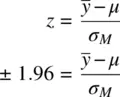
We can modify the equality slightly to get the following:

(2.3)

We interpret (2.3)as follows:

Over all possible samples, the probability is 0.95 that the range between and will include the true mean, μ.

Very important to note regarding the above statement is that μ is notthe random variable. The part that is random is the sample on which is computed the interval. That is, the probability statement is not about μ but rather is about samples. The population mean μ is assumed to be fixed. The 95% confidence interval tells us that if we continued to sample repeatedly, and on each sample computed a confidence interval, then 95% of these intervals would include the true parameter.

The 99% confidence interval for the mean is likewise given by:

(2.4)

Notice that the only difference between (2.3)and (2.4)is the choice of different critical values on either side of μ (i.e., 1.96 for the 95% interval and 2.58 for the 99% interval).

Though of course not very useful, a 100% confidence interval, if constructed, would be defined as:

If you think about it carefully, the 100% confidence interval should make perfect sense. If you would like to be 100% “sure” that the interval will cover the true population mean, then you have to extend your limits to negative and positive infinity, otherwise, you could not be fullyconfident. Likewise, on the other extreme, a 0% interval would simply have as the upper and lower limits:

That is, if you want to have zero confidencein guessing the location of the population mean, μ , then guess the sample mean . Though the sample mean is an unbiased estimator of the population mean, the probability that the sample mean covers the population mean exactly, as mentioned, essentially converges to 0 for a truly continuous distribution (Hays, 1994). As an analogy, imagine coming home and hugging your spouse. If your arms are open infinitely wide (full “bear hug”), you are 100% confident to entrap him or her in your hug because your arms (limits of the interval) extend to positive and negative infinity. If you bring your arms in a little, then it becomes possible to miss him or her with the hug (e.g., 95% interval). However, the precision of the hug is a bit more refined (because your arms are closing inward a bit instead of extending infinitely on both sides). If you approach your spouse with hands together (i.e., point estimate), you are sure to miss him or her, and would have 0% confidence of your interval (hug) entrapping your spouse. An inexact analogy to be sure, but useful in visualizing the concept of confidence intervals.