Daniel J. Denis - Applied Univariate, Bivariate, and Multivariate Statistics

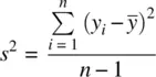
When we lose a degree of freedom in the denominator and rename S 2to s 2, we get

Recall that when we take the expectation of s 2, we find that E ( s 2) = σ 2(see Wackerly, Mendenhall, and Scheaffer (2002, pp. 372–373) for a proof).

The population standard deviationis given by the positive square root of σ 2, that is, . Analogously, the sample standard deviation is given by .

Recall the interpretation of a standard deviation. It tells us on average how much scores deviate from the mean. In computing a measure of dispersion, we initially squared deviations so as to avoid our measure of dispersion always equaling zero for any given set of observations, since the sum of deviations about the mean is always equal to 0. Taking the average of this sum of squares gave us the variance, but since this is in squared units, we wish to return them to “unsquared” units. This is how the standard deviation comes about. Studying the analysis of variance, the topic of the following chapter, will help in “cementing” some of these ideas of variance and the squaring of deviations, since ANOVA is all about generating different sums of squares and their averages, which go by the name of mean squares.

The variance and standard deviation are easily obtained in R. We compute for parent in Galton's data:

> var(parent) [1] 3.194561 > sd(parent) [1] 1.787333

One may also wish to compute what is known as the coefficient of variation, which is a ratio of the standard deviation to the mean. We can estimate this coefficient for parentand childrespectively in Galton's data:

> cv.parent <- sd(parent)/mean(parent) > cv.parent [1] 0.02616573 > cv.child <- sd(child)/mean(child) > cv.child [1] 0.03698044

Computing the coefficient of variation is a way of comparing the variability of competing distributions relative to each distribution's mean. We can see that the dispersion of child relative to its mean (0.037) is slightly larger than that of the dispersion of parent relative to its mean (0.026).

In our discussion of variance, we saw that if we wanted to use the sample variance as an estimator of the population variance, we needed to subtract 1 from the denominator. That is, S 2was “corrected” into s 2:

We say we lost a degree of freedomin the denominator of the statistic. But what are degrees of freedom? They are the number of independent units of information in a sample that are relevant to the estimation of some parameter(Everitt, 2002). In the case of the sample variance, s 2, one degree of freedom is lost since we are interested in using s 2as an estimator of σ 2. We are losing the degree of freedom because the numerator, , is not based on n independent pieces of information since μ had to be estimated by . Hence, a degree of freedom is lost. Why? Because values of y iare not independent of what is, since is fixed in terms of the given sample data. In general, when we estimate a parameter, it “costs” a degree of freedom. Had we μ , such that , we would have not lost a degree of freedom, since μ is a known (not estimated) parameter.

A conceptual demonstration may prove useful in understanding the concept of degrees of freedom. Imagine you were asked to build a triangle such that there was to be no overlap of lines on either side of the triangle. In other words, the lengths of the sides had to join neatly at the vertices. We shall call this the “ Beautiful Triangle” as depicted in Figure 2.9. You are now asked to draw the first side of the triangle. Why did you draw this first side the length that you did? You concede that the length of the first side is arbitrary, you were freeto draw it whatever length you wished. In drawing the second length, you acknowledge you were also freeto draw it whatever length you wished. Neither of the first two lengths in any way violated the construction of a beautiful triangle with perfectly adjoining vertices.

However, in drawing the third length, what length did you choose? Notice that to complete the triangle, you were not freeto determine this length arbitrarily. Rather, the length was fixedgiven the constraint that the triangle was to be a beautiful one. In summary then, in building the beautiful triangle, you lost 1 degree of freedom, in that two of the lengths were of your free choosing, but the third was fixed. Analogously, in using s 2as an estimator of σ 2, a single degree of freedom is lost. If is equal to 10, for instance, and the sample is based on five observations, then y 1, y 2, y 3, y 4are freely chosen, but the fifth data point, y 5is not freely chosen so long as the mean must equal 10. The fifth data point is fixed. We lost a single degree of freedom.

Figure 2.9The “Beautiful Triangle” as a way to understanding degrees of freedom.

Degrees of freedom occur throughout statistics in a variety of statistical tests. If you understand this basic example, then while working out degrees of freedom for more advanced designs and tests may still pose a challenge, you will nonetheless have a conceptual base from which to build your comprehension.

The third moment of a distribution is its skewness. Skewness of a random variable generally refers to the extent to which a distribution lacks symmetry. Skewness is defined as:

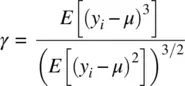
Skewness for a normal distribution is equal to 0, just as skewness for a rectangular distribution is also equal to 0 (one does not necessarily require a bell‐shaped curve for skewness to equal 0)