Daniel J. Denis - Applied Univariate, Bivariate, and Multivariate Statistics

When we speak of likelihood, we mean the probability of some sample data or set of observations conditional on some hypothesized parameter or set of parameters (Everitt, 2002). Conditional probability statements such as p ( D / H 0) can very generally be considered simple examples of likelihoods, where typically the set of parameters, in this case, may be simply μ and σ 2. A likelihood functionis the likelihood of a parameter given data (see Fox, 2016).

When we speak of maximum‐likelihoodestimation, we mean the process of maximizing a likelihood subject to certain parameter conditions. As a simple example, suppose we obtain 8 heads on 10 flips of a presumably fair coin. Our null hypothesis was that the coin is fair, meaning that the probability of heads is p ( H ) = 0.5. However, our actual obtained result of 8 heads on 10 flips would suggest the true probability of heads to be closer to p ( H ) = 0.8. Thus, we ask the question:

Which value of θ makes the observed result most likely?

If we only had two choices of θ to select from, 0.5 and 0.8, our answer would have to be 0.8, since this value of the parameter θ makes the sample result of 8 heads out of 10 flips most likely. That is the essence of how maximum‐likelihood estimation works (see Hays, 1994, for a similar example). ML is the most common method of estimating parameters in many models, including factor analysis, path analysis, and structural equation models to be discussed later in the book. There are very good reasons why mathematical statisticians generally approve of maximum likelihood. We summarize some of their most favorable properties.

Firstly, ML estimators are asymptotically unbiased, which means that bias essentially vanishes as sample size increases without bound (Bollen, 1989). Secondly, ML estimators are consistentand asymptotically efficient, the latter meaning that the estimator has a small asymptotic variance relative to many other estimators. Thirdly, ML estimators are asymptotically normally distributed, meaning that as sample size grows, the estimator takes on a normal distribution. Finally, ML estimators possess the invarianceproperty (see Casella and Berger, 2002, for details).

A measure of model fit commonly used in comparing models that uses the log‐likelihood is Akaike's information criteria, or AIC(Sakamoto, Ishiguro, and Kitagawa, 1986). This is one statistic of the kind generally referred to as penalized likelihoodstatistics (another is the Bayesian information criterion, or BIC). AIC is defined as:

where L mis the maximized log‐likelihood and m is the number of parameters in the given model. Lower values of AIC indicate a better‐fitting model than do larger values. Recall that the more parameters fit to a model, in general, the better will be the fit of that model. For example, a model that has a unique parameter for eachdata point would fit perfectly. This is the so‐called saturatedmodel. AIC jointly considers both the goodness of fit as well as the number of parameters required to obtain the given fit, essentially “penalizing” for increasing the number of parameters unless they contribute to model fit. Adding one or more parameters to a model may cause −2 L mto decrease (which is a good thing substantively), but if the parameters are not worthwhile, this will be offset by an increase in 2 m .

The Bayesian information criterion, or BIC(Schwarz, 1978) is defined as −2 L m+ m log( N ), where m , as before, is the number of parameters in the model and N the total number of observations used to fit the model. Lower values of BIC are also desirable when comparing models. BIC typically penalizes model complexity more heavily than AIC. For a comparison of AIC and BIC, see Burnham and Anderson (2011).

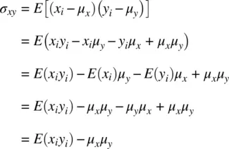
The covariance of a random variable is given by:

where E [( x i− μ x)( y i− μ y)] is equal to E ( x i y i) − μ x μ ysince

The concept of covariance is at the heart of virtually all statistical methods. Whether one is running analysis of variance, regression, principal component analysis, etc. covariance concepts are central to all of these methodologies and even more broadly to science in general.

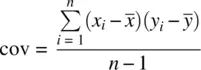
The sample covariance is a measure of relationship between two variables and is defined as:

(2.5)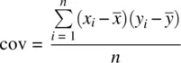

The numerator of the covariance, 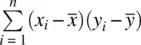, is the sum of products of respective deviations of observations from their respective means. If there is no linearrelationship between two variables in a sample, covariance will equal 0. If there is a negativelinear relationship, covariance will be a negative number, and if there is a positivelinear relationship covariance will be positive. Notice that to measure covariance between two variables requires there to be variabilityon each variable. If there is no variability in x i, then will equal 0 for all observations. Likewise, if there is no variability in y i, then will equal 0 for all observations on y i. This is to emphasize the essential fact that when measuring the extent of relationship between two variables, one requires variability on each variable to motivate a measure of relationship in the first place.

The covariance of (2.5)is a perfectly reasonable one to calculate for a sample if there is no intention of using that covariance as an estimator of the population covariance. However, if one wishes to use it as an unbiased estimator, similar to how we needed to subtract 1 from the denominator of the variance, we lose 1 degree of freedom when computing the covariance:

It is easy to understand more of what the covariance actually measures if we consider the trivial case of computing the covariance of a variable with itself. In such a case for variable x i, we would have