Daniel J. Denis - Applied Univariate, Bivariate, and Multivariate Statistics

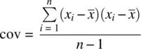
But what is this covariance? If we rewrite the numerator as instead of , it becomes clear that the covariance of a variable with itself is nothing more than the usual variancefor that variable. Hence, to better understand the covariance, it is helpful to start with the variance, and then realize that instead of computing the cross‐product of a variable with itself, the covariance computes the cross‐product of a variable with a secondvariable.

We compute the covariance between parent height and child height in Galton's data:

> attach(Galton) > cov(parent, child) [1] 2.064614

We have mentioned that the covariance is a measure of linear relationship. However, sample covariances from data set to data set are not comparable unless one knows more of what went into each specific computation. There are actually three things that can be said to be the “ingredients” of the covariance. The first thing it contains is a measure of the cross‐product, which represents the degree to which variables are linearly related. This is the part in our computation of the covariance that we are especially interested in. However, other than concluding a negative, zero, or positive relationship, the size of the covariance does not by itself tell us the degreeto which two variables are linearly related.

The reason for this is that the size of covariance will also be impacted by the degree to which there is variability in x iand the degree to which there is variability in y i. If either or both variables contain sizeable deviations of the sort or , then the corresponding cross‐products will also be quite sizeable, along with their sum, 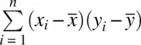. However, we do not want our measure of relationship to be small or large as a consequence of variability on x ior variability on y i. We want our measure of relationship to be small or large as an exclusive result of covariability, that is, the extent to which there is actually a relationshipbetween x iand y i. To incorporate the influences of variability in x iand y i(one may think of it as “purifying”), we divide the average cross‐product (i.e., the covariance) by the product of standard deviations of each variable. The standardized sample covarianceis thus:

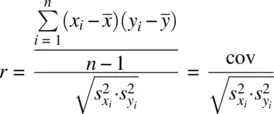
The standardized covariance is known as the Pearson product‐moment correlation coefficient, or simply r , which is a biasedestimator of its population counterpart, ρ xy, except when ρ xyis exactly equal to 0. The bias of the estimator r can be minimized by computing an adjustment found in Rencher (1998, p. 6), originally proposed by Olkin and Pratt (1958):

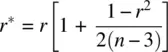
Because the correlation coefficient is standardized, we can place lower and upper bounds on it. The minimum the correlation can be for any set of data is −1.0, representing a perfect negative relationship. The maximum the correlation can be is +1.0, representing a perfect positive relationship. A correlation of 0 represents the absence of a linearrelationship. For further discussion on how the Pearson correlation can be a biased estimate under conditions of nonnormality (and potential solutions), see Bishara and Hittner (2015).

One can gain an appreciation for the upper and lower bound of r by considering the fact that the numerator, which is an average cross‐product, is being divided by another product, that of the standard deviations of each variable. The denominator thus can be conceptualized to represent the total amount of cross‐product variation possible, that is, the “base,” whereas the numerator represents the total amount of cross‐product variation actually existing between the variables because of a linear relationship. The extent to which cov xyaccounts for all of the possible “cross‐variation” in is the extent to which r will approximate a value of |1| (either positive or negative, depending on the direction of the relationship). It thus stands that cov xycannot be greater than the “base” to which it is being compared (i.e., ). In the language of sets, cov xymust be a subsetof the larger set represented by .

It is important to emphasize that a correlation of 0 does not necessarily represent the absenceof a relationship. What it does represent is the absence of a linearone. Neither the covariance or Pearson's r capture nonlinear relationships, and so it is possible to have very strong relations in a sample or population yet still obtain very low values (even zero) for the covariance or Pearson r . Always plot your data to see what is going on before drawing any conclusions. Correlation coefficients should never be presented without an accompanying plot to characterize the form of the relationship.

We compute the Pearson correlation coefficient on Galton's data between childand parent:

> cor(child, parent) [1] 0.4587624

We can test it for statistical significance by using the cor.testfunction:

> cor.test(child, parent) Pearson's product-moment correlation data: child and parent t = 15.7111, df = 926, p-value < 2.2e-16 alternative hypothesis: true correlation is not equal to 0 95 percent confidence interval: 0.4064067 0.5081153 sample estimates: cor 0.4587624

We can see that observed t is statistically significant with a computed 95% confidence interval having limits 0.41 to 0.51, indicating that we can be 95% confident that the true parameter lies approximately between the limits of 0.41 and 0.51. Using the package ggplot2(Wickham, 2009), we plot the relationship between parent and child (with a smoother):