Daniel J. Denis - Applied Univariate, Bivariate, and Multivariate Statistics

> iq <- c(105, 98, 110, 105, 95) > t.test(iq, mu = 100) One Sample t-test data: iq t = 0.965, df = 4, p-value = 0.3892 alternative hypothesis: true mean is not equal to 100 95 percent confidence interval: 95.11904 110.08096 sample estimates: mean of x 102.6

Just as the t ‐test for one sample is a generalization of the z ‐test for one sample, for which we use s 2in place of σ 2, the t ‐test for two independent samples is a generalization of the z ‐test for two independent samples. Recall the z ‐test for two independent samples:

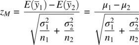
where and denote the expectations of the sample means and respectively (which are equal to μ 1and μ 2).

When we do not know the population variances and , we shall, as before, obtain estimates of them in the form of and . When we do so, because we are using these estimates instead of the actual variances, our new ratio is no longer distributed as z . Just as in the one‐sample case, it is now distributed as t :

(2.6)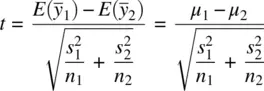

on degrees of freedom v = n 1− 1 + n 2− 1 = n 1+ n 2− 2.

The formulization of t in (2.6)assumes that n 1= n 2. If sample sizes are unequal, then poolingvariances is recommended. To pool, we weight the sample variances by their respective sample sizes and obtain the following estimated standard error of the difference in means:

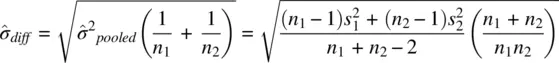
which can also be written as

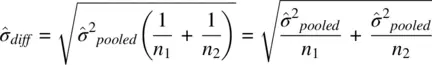
Notice that the pooled estimate of the variance 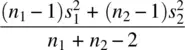is nothing more than an averaged weighted sum, each variance being weighted by its respective sample size. This idea of weighting variances as to arrive at a pooled value is not unique to t ‐tests. Such a concept forms the very fabric of how MS error is computed in the analysis of variance as we shall see further in Chapter 3when we discuss the ANOVA procedure in some depth.

Consider the following hypothetical data on pass‐fail grades (“0” is fail, “1” is pass) for a seminar course with 10 attendees:

grade studytime 0 30 0 25 0 59 0 42 0 31 1 140 1 90 1 95 1 170 1 120

To conduct the two‐sample t ‐test, we generate the relevant vectors in R then carry out the test:

> grade.0 <- c(30, 25, 59, 42, 31) > grade.1 <- c(140, 90, 95, 170, 120) > t.test(grade.0, grade.1) Welch Two Sample t-test data: grade.0 and grade.1 t = -5.3515, df = 5.309, p-value = 0.002549 alternative hypothesis: true difference in means is not equal to 0 95 percent confidence interval: -126.00773 -45.19227 sample estimates: mean of x mean of y 37.4 123.0

Using a Welch adjustmentfor unequal variances (Welch, 1947) automatically generated by R, we conclude a statistically significant difference between means ( p = 0.003). With 95% confidence, we can say the true mean difference lies between the lower limit of approximately −126.0 and the upper limit of approximately −45.2. As a quick test to verify the assumption of equal variances (and to confirm in a sense whether the Welch adjustment was necessary), we can use var.testwhich will produce a ratio of variances and evaluate the null hypothesis that this ratio is equal to 1 (i.e., if the variances are equal, the numerator of the ratio will be the same as the denominator):

> var.test(grade.0, grade.1) F test to compare two variances data: grade.0 and grade.1 F = 0.1683, num df = 4, denom df = 4, p-value = 0.1126 alternative hypothesis: true ratio of variances is not equal to 1 95 percent confidence interval: 0.01752408 1.61654325 sample estimates: ratio of variances 0.1683105

The var.testyields a p ‐value of 0.11, which under most circumstances would be considered insufficient reason to doubt the null hypothesis of equal variances. Hence, the Welch adjustment on the variances was probably not needed in this case as there was no evidence of an inequality of variances to begin with.

Carrying out the same test in SPSS is straightforward by requesting (output not shown):

t-test groups = grade(0 1) /variables = studytime.

A classic nonparametricequivalent to the independent‐samples t ‐test is the Wilcoxon rank‐sumtest. It is a useful test to run when either distributional assumptions are known to be violated or when they are unknown and sample size too small for the central limit theorem to come to the “rescue.” The test compares rankingsacross the two samples instead of actual scores. For a brief overview of how the test works, see Kirk (2008, Chapter 18) and Howell (2002, pp. 707–717), and for a more thorough introduction to nonparametric tests in general, see the following chapter on ANOVA in this book, or consult Denis (2020) for a succinct chapter and demonstrations using R. We can request the test quite easily in R:

> wilcox.test(grade.0, grade.1) Wilcoxon rank sum test data: grade.0 and grade.1 W = 0, p-value = 0.007937 alternative hypothesis: true location shift is not equal to 0

We see that the obtained p ‐value still suggests we reject the null hypothesis, though the p ‐value is slightly larger than for the Welch‐corrected parametric test.

Power, first and foremost, is a probability. Power is the probability of rejecting a null hypothesis given that the null hypothesis is false. It is equal to 1 − β (i.e., 1 minus the type II error rate). If the null hypothesis were true, then regardless of how much power one has, one would still not be able to reject the null. We may think of it somewhat in terms of the sensitivityof a statistical test for detecting the falsity of the null hypothesis. If the test is not very sensitive to departures from the null (i.e., in terms of a particular alternative hypothesis), we will not detect such departures. If the test is very sensitive to such departures, then we will correctly detect these departures and be able to infer the statistical alternative hypothesis in question.