Applied Modeling Techniques and Data Analysis 2

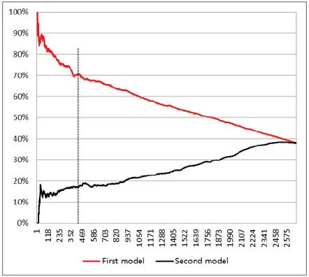
Figure 1.10. Coercive procedures’ rates. For a color version of this figure, see www.iste.co.uk/dimotikalis/analysis2.zip

This is just an example and it is not the only way we can combine the two models. Indeed, there is space for policymakers to exploit the two models in different ways, depending on the kind of tradeoff choices they may want to reach, concerning the two goals of the audit process: its profitability and its tax collectability. For instance, a selection process could only be targeted towards interesting taxpayers and taxpayers without payment issues.

Anyway, does the tradeoff we have sketched above work?

Figures 1.11- 1.13can shed some light on our ensemble model’s performance. As usual, the dashed vertical line shows the values corresponding to the number of taxpayers we wish to select.

In our case, thus, with the ensemble model , we would claim, on average, € 26,219 from the selected taxpayers and we would hopefully collect, on average, € 17,542 from each of them, of whom only 25% are predicted to incur in coercive procedures.

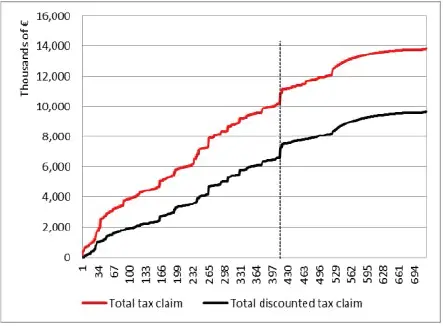
Figure 1.11. Total tax claim. For a color version of this figure, see www.iste.co.uk/dimotikalis/analysis2.zip

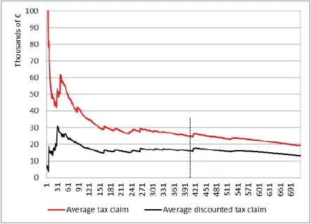
Figure 1.12. Average tax claim. For a color version of this figure, see www.iste.co.uk/dimotikalis/analysis2.zip

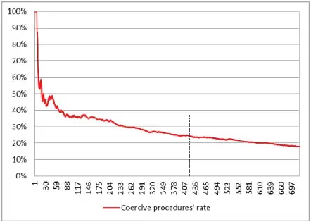
Figure 1.13. Coercive procedures’ rate. For a color version of this figure, see www.iste.co.uk/dimotikalis/analysis2.zip

In a hypothetical selection process, the winning strategy would then be to use the ensemble model , since it maximizes the collectable tax claim .

What we might be interested in, is to know whether the ensemble model is always the best option. This may depend on the coercive procedures’ rate that characterizes the two sets of auditable taxpayers selected by the two models. Unfortunately, once we build the models, before applying them to the test set, we do not exactly know what kind of taxpayers will be selected. Therefore, we do not even know these rates; however, we can consider them as unknown parameters, say θ’ and θ” . From this point of view, the rates we have observed within the two selected sets can be considered as two values of such parameters, say (70%) and (25%) (see Table 1.5).

To satisfy our interest, we should depict the two models’ behavior as a function of the unknown parameters, θ’ and θ” , respectively; that is, we should calculate the expected tax revenues amounts for any value of θ’ and θ” . Unfortunately, this cannot be done. To understand why, suppose that for both models, only one of the selected taxpayers turns out to be subject to coercive procedures. If this taxpayer’s debt is high, the amount of money that is difficult to collect would be high, but if his debt is low, then the uncollected tax would also be low.

What can be done, instead, is to calculate, for any given value of θ’ and θ” , the maximum and minimum collectable taxes arising from each model. Indeed, the maximum collectable taxes scenario is the one where coercive procedures are first applied to the less unfaithful taxpayers, while the minimum collectable taxes scenario refers to a situation in which coercive procedures are first applied to the most unfaithful taxpayers, as shown in Figure 1.14.

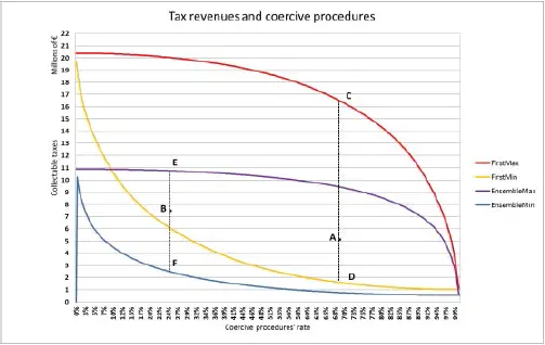
Figure 1.14. Models’ maximum and minimum collected tax. For a color version of this figure, see www.iste.co.uk/dimotikalis/analysis2.zip

The first model’s maximum and minimum values are represented by the red and orange lines, while the ensemble model’s are the blue and purple ones. Any point within the red and orange lines represents a possible outcome for the first model and any point within the blue and purple lines represents one possible outcome for the ensemble model . For instance, points A and B represent the outcomes of our models (the first and the ensemble , respectively), given our training and test sets.

Having to deal with two areas means that the models’ behavior is determined not only by θ’ and θ” , but also by the kind of taxpayers that go through a coercive procedure. If we could shrink the areas between the red and orange lines and the blue and purple ones, we could be put in a better shape.

How could we do this? Well, if we turn back to points A and B in Figure 1.14, and we draw two dashed vertical lines from them, we can see that the first is nearer to the minimum line of its model (since line is shorter than line ), while the other is nearer to the maximum one (since line is shorter than line ).

If we assume that, for each value of θ’ and θ” and for each corresponding points A (and, also, lines and ) and B (and, also, lines and ), ratios are always the same and also ratios , we could draw a single line for each model, which would only be a function of θ’ and θ’’ , respectively, as shown in Figure 1.15.