Applied Modeling Techniques and Data Analysis 2
Здесь есть возможность читать онлайн «Applied Modeling Techniques and Data Analysis 2» — ознакомительный отрывок электронной книги совершенно бесплатно, а после прочтения отрывка купить полную версию. В некоторых случаях можно слушать аудио, скачать через торрент в формате fb2 и присутствует краткое содержание. Жанр: unrecognised, на английском языке. Описание произведения, (предисловие) а так же отзывы посетителей доступны на портале библиотеки ЛибКат.
- Название:Applied Modeling Techniques and Data Analysis 2
- Автор:
- Жанр:
- Год:неизвестен
- ISBN:нет данных
- Рейтинг книги:5 / 5. Голосов: 1
-
Избранное:Добавить в избранное
- Отзывы:
-
Ваша оценка:
Applied Modeling Techniques and Data Analysis 2: краткое содержание, описание и аннотация
Предлагаем к чтению аннотацию, описание, краткое содержание или предисловие (зависит от того, что написал сам автор книги «Applied Modeling Techniques and Data Analysis 2»). Если вы не нашли необходимую информацию о книге — напишите в комментариях, мы постараемся отыскать её.
Applied Modeling Techniques and Data Analysis 2 — читать онлайн ознакомительный отрывок
Ниже представлен текст книги, разбитый по страницам. Система сохранения места последней прочитанной страницы, позволяет с удобством читать онлайн бесплатно книгу «Applied Modeling Techniques and Data Analysis 2», без необходимости каждый раз заново искать на чём Вы остановились. Поставьте закладку, и сможете в любой момент перейти на страницу, на которой закончили чтение.
Интервал:
Закладка:
Pagliarani and Pascucci (2012) derived a fully explicit approximation for the implied volatility at any given order N ≥ 0 for the scalar case. Lorig et al . (2017) extended this result to the multidimensional case. Denote the above approximation by  .
.
Pagliarani and Pascucci (2017) proved that under some mild conditions, the following limits exist:
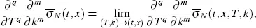
where the limit is taken as ( T,k ) approaches ( t,x ) within the parabolic region

for an arbitrary positive real number λ and nonnegative integers m and q .
Moreover, Pagliarani and Pascucci (2017) established an asymptotic expansion of the implied volatility in the following form:
[2.2] 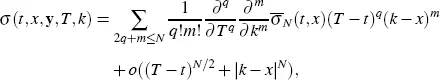
as ( T,k ) approaches ( t,x ) within  .
.
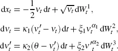
We apply the above described theory to the double-mean-reverting model by Gatheral (2008) given by the following system of stochastic differential equations:
[2.3] 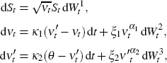
where the Wiener processes  are correlated:
 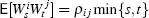 , and where parameters κ1,κ2, θ, ξ1, ξ2, α1, α2 are the positive real numbers. Note that while S 0is observable in the market, ν0 and
  are usually not observable and may be calibrated from the market data on options.
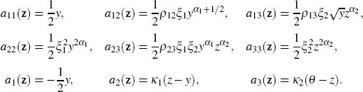
In this model, with rate κ 1the variance νt mean reverts to a level  which itself moves over time to the level θ at a (usually slower rate) κ2, hence the name double-mean-reverting. Here, parameters α1, α2 ∈ [1 / 2 , 1]. In the case of α1 = α2 = 1/2, we have the so-called double Heston model; in the case of α1 = α2 = 1, the double lognormal model; and finally, in the general case, the double CEV model (Gatheral 2008).
The DMR model can be consistently calibrated to both the SPX options and the VIX options. However, due to the lack of an explicit formula for both the European option price and the implied volatility, the calibration is usually done using time-consuming methods like the Monte Carlo simulation or the finite difference method. In this chapter, we provide an explicit solution to the implied volatility under this model.
In section 2.2, we formulate three theorems that give the asymptotic expansions of implied volatility of orders 0, 1 and 2. Detailed proof of Theorems 2.1 and 2.2 as well as a short proof of Theorem 2.3 without technicalities are given in section 2.3.
2.2. The results
Put xt = ln St .
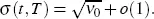
THEOREM 2.1.- The asymptotic expansion of order 0 of the implied volatility has the form
THEOREM 2.2.- The asymptotic expansion of order 1 of the implied volatility has the form

THEOREM 2.3.- The asymptotic expansion of order 2 of the implied volatility has the form
[2.4] 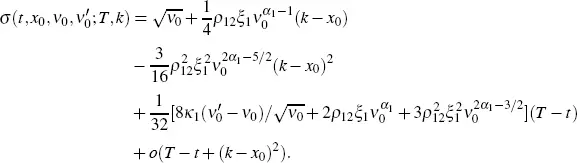
2.3. Proofs
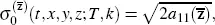
PROOF OF THEOREM 2.1.- First, we perform the change of variable χt = ln St in the system [2.3]. Using the multidimensional Itô formula, we obtain
The infinitesimal generator of this system is
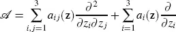
with z= ( x,y,z ) T. We have
From Pagliarani and Pascucci (2017), Definition 3.4, we have
[2.5] 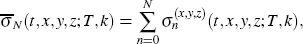
where the terms on the right-hand side of equation [2.5]are the values of the functions 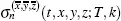 given by (Pagliarani and Pascucci 2017, Equation 3.15), when
  , and
, and  . (Pagliarani and Pascucci 2017, Equation 3.15) is recursive, and we define the above functions for n = 0 first.
Following Lorig et al . (2017), Appendix B, put  . From Lorig et al . (2017), Equation 3.2, we have
where  . It follows that
 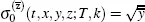 . Then, we have
Интервал:
Закладка:
Похожие книги на «Applied Modeling Techniques and Data Analysis 2»
Представляем Вашему вниманию похожие книги на «Applied Modeling Techniques and Data Analysis 2» списком для выбора. Мы отобрали схожую по названию и смыслу литературу в надежде предоставить читателям больше вариантов отыскать новые, интересные, ещё непрочитанные произведения.


Обсуждение, отзывы о книге «Applied Modeling Techniques and Data Analysis 2» и просто собственные мнения читателей. Оставьте ваши комментарии, напишите, что Вы думаете о произведении, его смысле или главных героях. Укажите что конкретно понравилось, а что нет, и почему Вы так считаете.