Anand K. Verma - Introduction To Modern Planar Transmission Lines

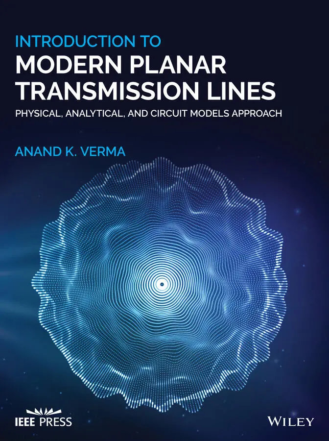
(4.7.21)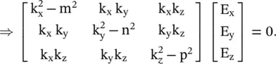

The nontrivial solution for E i(i = x, y, z) of the above homogeneous equation is det[ ] = 0, i.e.

(4.7.22)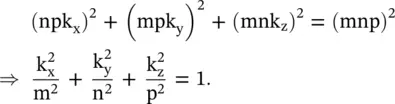

The above dispersion relation is a quadratic equation of any component of k 2. So, there are two solutions for any component of k. Two solutions correspond to two normal modes of propagation in the anisotropic medium. At a fixed frequency, equation (4.7.22)is the equation of an ellipsoid surface in the k‐space (wavevector space) , i.e. the normal space . For an isotropic medium, it is reduced to a sphere. Further, on knowing the wavenumber, the field components E i(i = x, y, z) can be determined from equation (4.7.21).

The discussion of dispersion in the uniaxial medium requires an understanding of the concept of isofrequency contours and isofrequency surfaces in the 2D and 3D k‐space. Figure (4.14a–d)explain the concept of isofrequency contours.

The wave propagation is considered in the isotropic (x‐y)‐plane. The dispersion relations for the 2D waves propagation in the isotropic medium and also in air medium are expressed as

(4.7.23)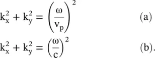

At a fixed frequency ω, the above equations are equations of circles in the (k x‐k y)‐plane. Figure (4.14a)shows that the radius of the circle increases with an increase in frequency. It forms a light cone . Figure (4.14b)further shows the increase in the 2D wavevector at the increasing order of frequencies ω 1< ω 2< ω 3< ω 4. The concentric contours of the wavevector are known as the isofrequency contours, displaying the dispersion relation. The light cone of the 2D dispersion diagram is generated by revolving Fig. ( 2.4) of the 1D dispersion diagram, shown in chapter 2, around the ω‐axis. Likewise, 3D isofrequency surfaces are obtained. It is discussed in the next section.

The propagating wave in the z‐direction is described by equation (4.7.12). The propagation constant 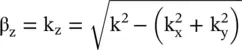of the waves must be real. So, the propagating waves are obtained only for 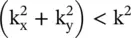, i.e. within the light cone. Outside the light cone, i.e. for 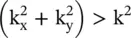, the waves are nonpropagating evanescent waves . Thus, the light cone divides the k‐space into the propagating and evanescent wave regions shown in Fig. (4.14a,c and d).

Further, any point P on the isofrequency contour surface, shown in Fig. (4.14b), connected to the origin O shows the direction of the wavevector. It is also the direction of the phase velocity v p. The direction of the normal at point P shows the direction of the Poynting vector, i.e. the direction of the group velocity v g. For an isotropic medium, both the v pand v gare in the same direction. It is noted that the wavefront is always normal to the wavevector . However, for the anisotropic medium, the phase and group velocities may not in the same direction. It is discussed below.

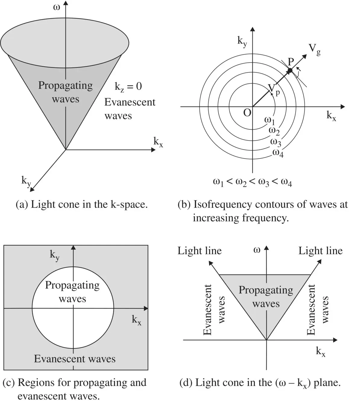
Figure 4.14 Dispersion diagrams of the wave propagating in the z‐direction in the isotropic medium.

This section considers the dispersion relation of a uniaxial anisotropic permittivity medium as a special case of the dispersion relation (4.7.19)of the biaxial medium. The permittivity along the optic axis, i.e. the z‐axis is ε zz= ε ‖and permeability of the medium is μ. The (x‐y)‐plane, with permittivity tensor elements ε xx= ε yy= ε ⊥, is a transverse plane. So, the medium is isotropic in the (x‐y)‐plane. The propagation constant along the z‐axis is k zand in the transverse plane, it is k t, satisfying the relation 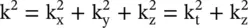. To simplify equation (4.7.19)for the uniaxial medium, the transverse wavevector in the (x‐y)‐plane is aligned such that the wave propagates only along the x‐axis, i.e. k y= 0 and k x= k t. Under such alignment, equation (4.7.19)is reduced to the following dispersion relation:

(4.7.24)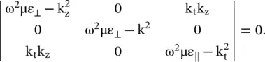

The above equation provides the following characteristic equation:

(4.7.25)

The above expression is also obtained from equation (4.7.19)even for the alignment of the wavevector to the y‐axis, i.e. k x= 0 and k y= k t. So, the characteristic equation (4.7.25)gives the following two independent dispersion relations:

(4.7.26)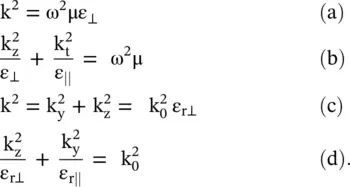

The above equations (4.7.26a)and (4.7.26b)demonstrate the presence of two normal modes of wave propagation in the 3D (k x, k y, k z) – space. Next, the 3D dispersion relation is reduced to the 2D dispersion relation given by equations (4.7.26c)and (4.7.26d). Equation (4.7.26a)is an equation of sphere in the 3D k‐space at a fixed frequency, i.e. at ω = constant. It shows the dispersion relation of the ordinary waves with the wavevector . At increasing order of frequencies, equation (4.7.26a)provides isofrequency spherical surfaces . Likewise, equation (4.7.26b)is an equation of ellipsoid in the 3D k‐space at a fixed frequency. It provides the dispersion relation of the extraordinary waves in the form of the concentric isofrequency ellipsoidal surfaces . The wavevector of extraordinary wave k eis rotation dependent.