Mantle Convection and Surface Expressions

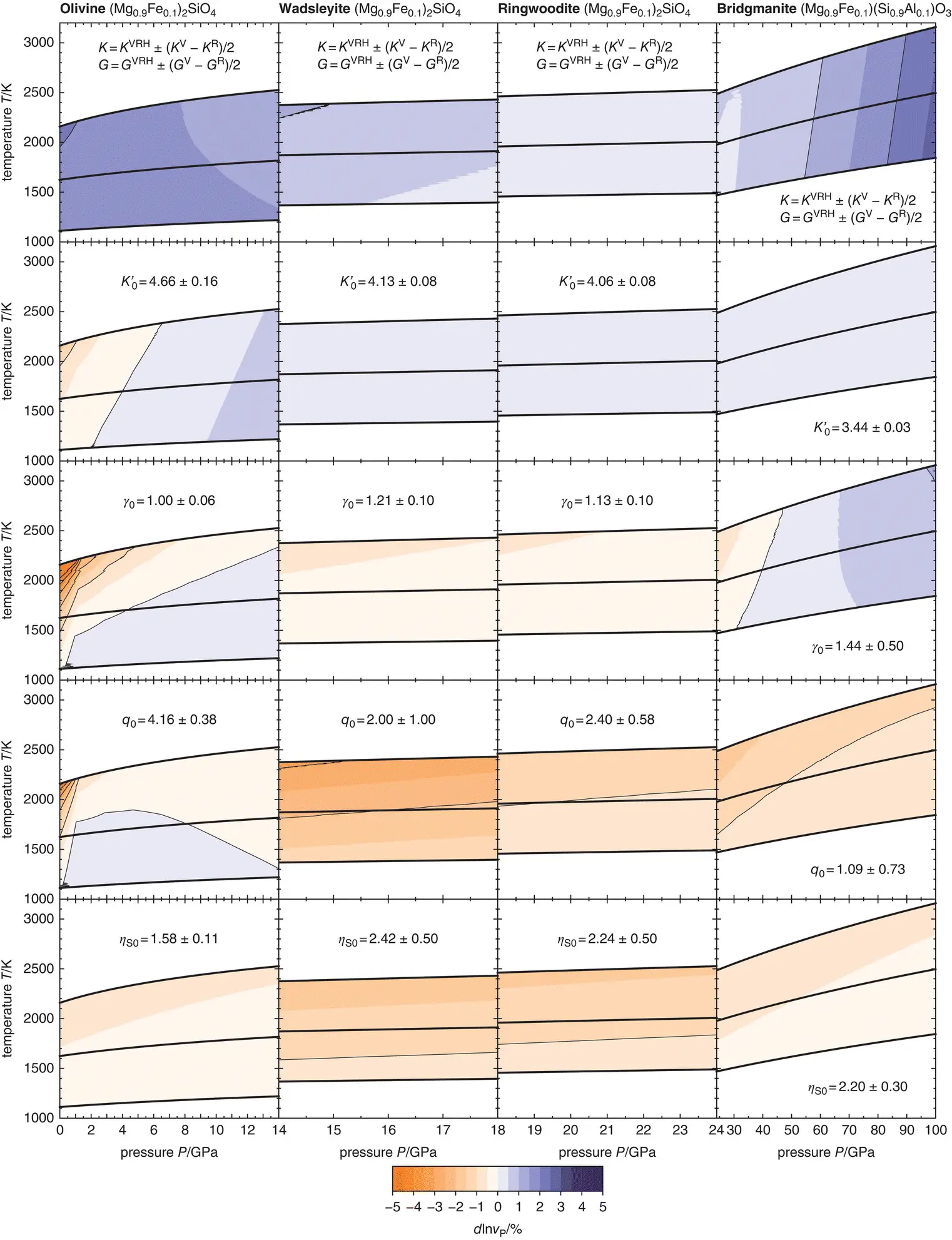
Figure 3.1 Variations in P‐ wave velocities for isotropic polycrystalline aggregates of olivine (1st column), wadsleyite (2nd column), ringwoodite (3rd column), and bridgmanite (4th column) that result from propagating uncertainties on individual finite‐strain parameters. Respective parameters and uncertainties are given in each panel. Bold black curves show adiabatic compression paths separated by temperature intervals of 500 K at the lowest pressure for each mineral. See text for references.

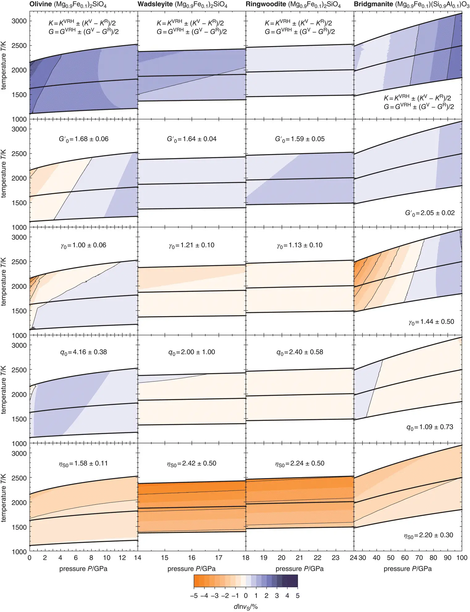
Figure 3.2 Variations in S‐ wave velocities for isotropic polycrystalline aggregates of olivine (1st column), wadsleyite (2nd column), ringwoodite (3rd column), and bridgmanite (4th column) that result from propagating uncertainties on individual finite‐strain parameters. Respective parameters and uncertainties are given in each panel. Bold black curves show adiabatic compression paths separated by temperature intervals of 500 K at the lowest pressure for each mineral. See text for references.

Most minerals form solid solutions spanned by two or more end members. When the molar or unit cell volumes Vi of the end members are known, a complex mineral composition given in terms of molar fractions x iof the end members is readily converted to volume fractions v i. Assuming ideal mixing behavior for volumes, the volume of the solid solution is then given by:

Based on the volume fractions v i= x i V i/ V , the elastic properties of end members can then be combined according to one of the averaging schemes introduced in Section 3.2to approximate the elastic behavior of the solid solution. Mineral‐physical databases compile elastic and thermodynamic properties for many end members of mantle minerals (Holland et al., 2013; Stixrude & Lithgow‐Bertelloni, 2011). However, the physical properties of some critical end members remain unknown, either because they have not been determined at relevant pressures and temperatures or because the end members are not stable as pure compounds.

Bridgmanite is believed to be the most abundant mineral in the lower mantle and adopts a perovskite crystal structure. Most bridgmanite compositions can be expressed as solid solutions of the end members MgSiO 3, FeSiO 3, Al 2O 3, and FeAlO 3. Of these end members, only MgSiO 3is known to have a stable perovskite‐structured polymorph at pressures and temperatures of the lower mantle. FeSiO 3perovskite is unstable with respect to the post‐perovskite form of FeSiO 3or a mixture of the oxides FeO and SiO 2(Caracas and Cohen, 2005; Fujino et al., 2009). Al 2O 3transforms from corundum to a Rh 2O 3(II) structured polymorph instead of adopting a perovskite structure (Funamori and Jeanloz, 1997; Kato et al., 2013; Lin et al., 2004). For FeAlO 3, both perovskite and Rh 2O 3(II) structures have been proposed (Caracas, 2010; Nagai et al., 2005). Although first‐principle calculations can access the elastic properties of compounds in thermodynamically unstable structural configurations, for example for FeSiO 3and Al 2O 3in perovskite structures (Caracas & Cohen, 2005; Muir & Brodholt, 2015a; Stackhouse et al., 2005a, 2006), it is unclear to which extent the results are useful for modeling the elastic properties of complex solid solutions that do not extend towards those end member compositions and might be affected by deviations from ideal mixing behavior at intermediate compositions.

When the physical properties of end members are unknown, it might still be possible to approximate the elastic properties of a solid solution as long as the effects of different chemical substitutions on elastic properties are captured by available experiments or computations on intermediate compositions of the solid solution. Let x imbe the molar fractions of end member i for a set of intermediate compositions for which volumes and elastic properties are known. For each composition m of this set, the molar fractions x imof all end members form a composition vector x mof dimension n equal to the total number of end members. If the set of compositions x mforms a vector basis of ℝ n, it is possible to construct a matrix M { x im} that contains the vectors x mas columns. Any composition vector xof the solid solution can then be transformed into a vector yby using the inverse matrix: y= M −1 x. The components of the vector yexpress the composition xin terms of molar fractions y mof the intermediate compositions x m. In this way, the compositions x mare combined to match the required composition, and their volumes and elastic properties can be combined according to the mixing laws introduced above. It is important to note that this type of mixing is strictly valid only within the compositional limits defined by the compositions x mthat may not cover the full compositional space as spanned by the end members. When volumes can be assumed to mix linearly across the entire solid solution, however, it is possible to extrapolate volumes beyond these compositional limits. The extrapolation of elastic properties requires special caution since negative molar fractions y m< 0 can lead to unwanted effects when computing bounds on elastic moduli.

Figure 3.3illustrates the uncertainties that arise from mixing the elastic properties of bridgmanite compositions. P‐ and S‐ wave velocities were calculated for bridgmanite solid solutions in the systems MgSiO 3‐Al 2O 3‐FeAlO 3and MgSiO 3‐Al 2O 3‐FeSiO 3at 40 GPa and 2000 K using available high‐pressure experimental data on different bridgmanite compositions (Chantel et al., 2012; Fu et al., 2018; Kurnosov et al., 2017; Murakami et al., 2012, 2007) that provided the basis of composition vectors in the approach outlined in the previous paragraph. For all compositions, I adopted the thermoelastic properties given by Zhang et al. (2013). Uncertainties on P‐ and S‐ wave velocities due to mixing were estimated as the differences that arise from combining the elastic properties of bridgmanite compositions according to either the Voigt or the Reuss bound relative to velocities of the Voigt‐Reuss‐Hill average, i.e., d ln v = ( v V− v R)/ v VRH. For bridgmanite compositions that are similar to the compositions studied in experiments and used here to compute P‐ and S‐ wave velocities, the uncertainties remain below 0.5%. When extrapolating elastic properties beyond the compositional limits defined by available experimental data, however, uncertainties rise substantially. Note that bridgmanite compositions falling outside the compositional range as delimited by experiments imply negative molar fractions in terms of the experimental compositions that form the basis of composition vectors. As a result, the Reuss bound may exceed the Voigt bound and d ln v < 0. As mentioned above, such extrapolations may exert strong leverages on sound wave velocities and need to be restricted to compositions that remain close to the compositional limits defined by available data.