Computational Analysis and Deep Learning for Medical Care

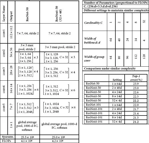
The ResNeXt [7] architecture is built based on the advantages of ResNet (residual networks) and GoogleNet (multi-branch architecture) and requires less number of hyperparameters compared to the traditional ResNet. The next defines the next dimension (“ cardinality ”), an additional dimension on top of the depth and width of ResNet. The input is split channelwise into groups. The standard residual block is replaced with a “ split-transform-merge ” procedure. This architecture uses a series of residual blocks and uses the following rules. (1) If the spatial maps are of same size, the blocks will split the hyperparameters; (2) The spatial map is pooled by two factors; block width is doubled by two factors. ResNeXt becomes the 1 strunner up of ILSVRC classification task and produces better results than ResNet. Figure 1.8shows the architecture of ResNeXt, and the comparison with REsNet is shown in Table 1.8.

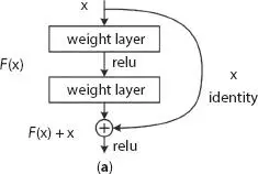
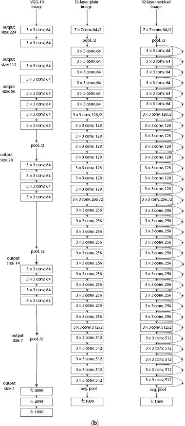
Figure 1.7 (a) A residual block.

Table 1.7 Various parameters of ResNet.

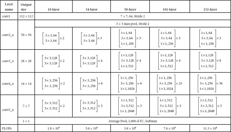
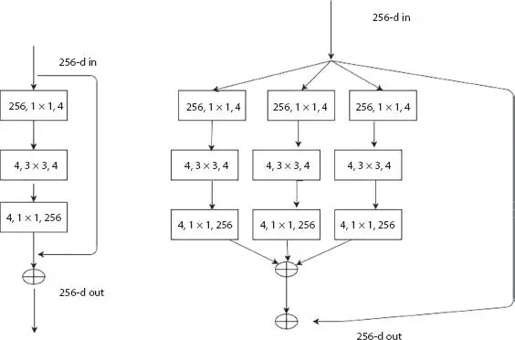
Figure 1.8 Architecture of ResNeXt.

Hu et al . [8] proposed a Squeeze-and-Excitation Network (SENet) (first position on ILSVRC 2017 category) with lightweight gating mechanism. This architecture focuses explicitly on model interdependencies between the channels of convolutional features and to achieve dynamic channel-wise feature recalibration. In the squeeze phase, SE block uses global average pooling operation and in the excitation phase uses channel-wise scaling. For an input image of size 224 × 224, the running time of ResNet-50 is 164 ms, whereas it is 167 ms for SE-ResNet-50. Also, SE-ResNet-50 requires ∼3.87 GFLOPs, which shows a 0.26% relative increase over the original ResNet-50. The top-5 error is reduced to 2.251%. Figure 1.9shows the architecture of SE-ResNet, and Table 1.9shows ResNet and its comparison with SE-ResNet-50 and SE-ResNeXt-50.

The architecture is proposed by [9], where every layer connect directly with each other so as to ensure maximum information (and gradient) flow. Thus, this model with L layer has L(L+1) connections. A number of dense block (group of layers connected to previous layers) and the transition layer control the complexity of the model. Each dense block adds one channel to the model. Transition layer is used to reduce the number of channels by using the convolutional layer of size 1 × 1 and reduces the width and height of the average pooling layer by a factor of 2 and with a stride of 2. It concatenates all the output feature map of previous layers along with incoming feature maps, i.e., each layer has direct access to the gradients from the loss function and the original input image. Further, DenseNets needs small set of parameters as compared to the traditional CNN and reduces vanishing gradient problem. Figure 1.10shows the architecture of DenseNet, and Table 1.10shows various DenseNet architectures.

Table 1.8 Comparison of ResNet-50 and ResNext-50 (32 × 4d).

Google proposed MobileNets VI [10] uses depthwise separable convolution instead of the normal convolutions, which, in turn, reduces the model size and complexity. Depthwise separable convolution is defined as a depthwise convolution followed by a pointwise convolution, i.e., a single convolution is performed on each colour channel and it is followed by pointwise convolution which applies a 1 × 1 convolution to combine the outputs of depthwise convolution; after each convolution, batch normalization (BN) and ReLU are applied. The whole architecture consists of 30 layers with (1) Convolutional layer with stride 2, (2) Depthwise layer, (3) Pointwise layer, (4) Depthwise layer with stride 2, and (5) Pointwise layer. The advantage of MobileNets is that it requires fewer number of parameters and the model is less complex (small number of Multiplications and Additions). Figure 1.11shows the architecture of MobileNets. Table 1.11shows the various parameters of MobileNets.

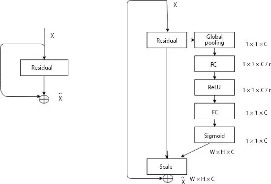
Figure 1.9 Architecture of SE-ResNet.

Mader [11] proposed V-Net for the detection of IVD. Bateson [12] propose a method which embeds domain-invariant prior knowledge and employ ENet to segment IVD. Other works which deserve special mentioning for the detection and segmentation of IVD from a 3D Spine MRI includes Zeng [13] uses CNN; Chang Liu [14] utilized 2.5D multi-scale FCN; Gao [15] presented a 2D CNN and DenseNet; Jose [17] presents a HD-UNet asym model; and Claudia Iriondo [16] uses VNet-based 3D connected component analysis algorithm.

Table 1.9 Comparison of ResNet-50 and ResNext-50 and SE-ResNeXt-50 (32 × 4d).

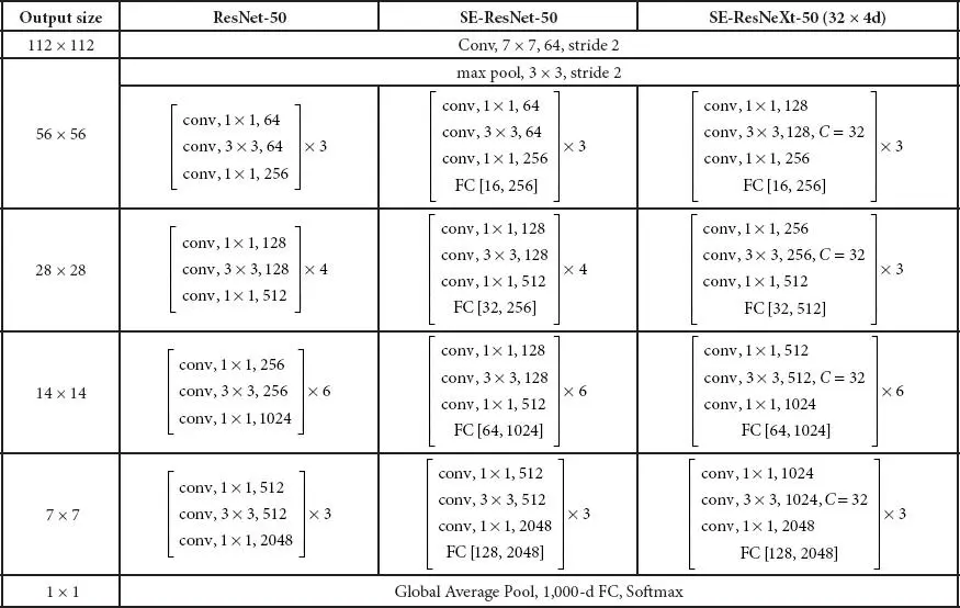
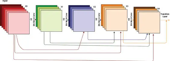
Figure 1.10 Architecture of DenseNet.

This work discusses the various architecture of CNN that have been employed for the segmentation of spine MRI. The difference in the architecture depends on several factors like number of layers, number of filters, whether padding is required or not, and the presence or absence of striding. The performance of segmentation is evaluated using Dice Similarity Coefficient (DSC), Mean Absolute Surface Distance (MASD), etc., and the experimental results are shown in Table 1.12. In the first three literature works, DSC is computed and CNN developed by Zeng et al . achieves 90.64%. DenseNET produces approximately similar segmentations based on MASD, Mean Localisation Distance (MLD), and Mean Dice Similarity Coefficient (MDSC). Comparison result is shown in Table 1.12.

In this Chapter, we had discussed about the various CNN architectural models and its parameters. In the first phase, various architectures such as LeNet, AlexNet, VGGnet, GoogleNet, ResNet, ResNeXt, SENet, and DenseNet and MobileNet are studied. In the second phase, the application of CNN for the segmentation of IVD is presented. The comparison with state-of-the-art of segmentation approaches for spine T2W images are also presented. From the experimental results, it is clear that 2.5D multi-scale FCN outperforms all other models. As a future study, this work modify any currents models to get optimized results.