Computational Analysis and Deep Learning for Medical Care
Здесь есть возможность читать онлайн «Computational Analysis and Deep Learning for Medical Care» — ознакомительный отрывок электронной книги совершенно бесплатно, а после прочтения отрывка купить полную версию. В некоторых случаях можно слушать аудио, скачать через торрент в формате fb2 и присутствует краткое содержание. Жанр: unrecognised, на английском языке. Описание произведения, (предисловие) а так же отзывы посетителей доступны на портале библиотеки ЛибКат.
- Название:Computational Analysis and Deep Learning for Medical Care
- Автор:
- Жанр:
- Год:неизвестен
- ISBN:нет данных
- Рейтинг книги:5 / 5. Голосов: 1
-
Избранное:Добавить в избранное
- Отзывы:
-
Ваша оценка:
Computational Analysis and Deep Learning for Medical Care: краткое содержание, описание и аннотация
Предлагаем к чтению аннотацию, описание, краткое содержание или предисловие (зависит от того, что написал сам автор книги «Computational Analysis and Deep Learning for Medical Care»). Если вы не нашли необходимую информацию о книге — напишите в комментариях, мы постараемся отыскать её.
Computational Analysis and Deep Learning for Medical Care — читать онлайн ознакомительный отрывок
Ниже представлен текст книги, разбитый по страницам. Система сохранения места последней прочитанной страницы, позволяет с удобством читать онлайн бесплатно книгу «Computational Analysis and Deep Learning for Medical Care», без необходимости каждый раз заново искать на чём Вы остановились. Поставьте закладку, и сможете в любой момент перейти на страницу, на которой закончили чтение.
Интервал:
Закладка:
ZFNet uses cross-entropy loss error function, ReLU activation function, and batch stochastic gradient descent. Training is done on 1.3 million images uses a GTX 580 GPU and it takes 12 days. The ZFNet architecture consists of five convolutional layers, followed by three max-pooling layers, and then by three fully connected layers, and a softmax layer as shown in Figure 1.3. Table 1.4shows an input image 224 × 224 × 3 and it is processing at each layer and shows the filter size, window size, stride, and padding values across each layer. ImageNet top-5 error improved from 16.4% to 11.7%.
1.2.4 VGGNet
Simonyan and Zisserman et al . [4] introduced VGGNet for the ImageNet Challenge in 2014. VGGNet-16 consists of 16 layers; accepts a 227 × 227 × 3 RGB image as input, by subtracting global mean from each pixel. Then, the image is fed to a series of convolutional layers (13 layers) which uses a small receptive field of 3 × 3 and uses same padding and stride is 1. Besides, AlexNet and ZFNet uses max-pooling layer after convolutional layer. VGGNet does not have max-pooling layer between two convolutional layers with 3 × 3 filters and the use of three of these layers is more effective than a receptive field of 5 × 5 and as spatial size decreases, the depth increases. The max-pooling layer uses a window of size 2 × 2 pixel and a stride of 2. It is followed by three fully connected layers; first two with 4,096 neurons and third is the output layer with 1,000 neurons, since ILSVRC classification contains 1,000 channels. Final layer is a softmax layer. The training is carried out on 4 Nvidia Titan Black GPUs for 2–3 weeks with ReLU nonlinearity activation function. The number of parameters is decreased and it is 138 million parameters (522 MB). The test set top-5 error rate during competition is 7.1%. Figure 1.4shows the architecture of VGG-16, and Table 1.5shows its parameters.
Table 1.4 Various parameters of ZFNet.
| Layer name | Input size | Filter size | Window size | # Filters | Stride | Padding | Output size | # Feature maps | # Connections |
| Conv 1 | 224 × 224 | 7 × 7 | - | 96 | 2 | 0 | 110 × 110 | 96 | 14,208 |
| Max-pooling 1 | 110 × 110 | 3 × 3 | - | 2 | 0 | 55 × 55 | 96 | 0 | |
| Conv 2 | 55 × 55 | 5 × 5 | - | 256 | 2 | 0 | 26 × 26 | 256 | 614,656 |
| Max-pooling 2 | 26 × 26 | - | 3 × 3 | - | 2 | 0 | 13 × 13 | 256 | 0 |
| Conv 3 | 13 × 13 | 3 × 3 | - | 384 | 1 | 1 | 13 × 13 | 384 | 885,120 |
| Conv 4 | 13 × 13 | 3 × 3 | - | 384 | 1 | 1 | 13 × 13 | 384 | 1,327,488 |
| Conv 5 | 13 × 13 | 3 × 3 | - | 256 | 1 | 1 | 13 × 13 | 256 | 884,992 |
| Max-pooling 3 | 13 × 13 | - | 3 × 3 | - | 2 | 0 | 6 × 6 | 256 | 0 |
| Fully connected 1 | 4,096 neurons | 37,752,832 | |||||||
| Fully connected 2 | 4,096 neurons | 16,781,312 | |||||||
| Fully connected 3 | 1,000 neurons | 4,097,000 | |||||||
| Softmax | 1,000 classes | 62,357,608 (Total) |
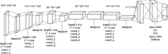
Figure 1.4 Architecture of VGG-16.
1.2.5 GoogLeNet
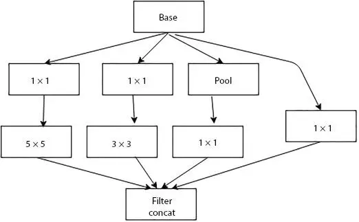
In 2014, Google [5] proposed the Inception network for the ImageNet Challenge in 2014 for detection and classification challenges. The basic unit of this model is called “Inception cell”—parallel convolutional layers with different filter sizes, which consists of a series of convolutions at different scales and concatenate the results; different filter sizes extract different feature map at different scales. To reduce the computational cost and the input channel depth, 1 × 1 convolutions are used. In order to concatenate properly, max pooling with “same” padding is used. It also preserves the dimensions. In the state-of-art, three versions of Inception such as Inception v2, v3, and v4 and Inception-ResNet are defined. Figure 1.5shows the inception module and Figure 1.6shows the architecture of GoogLeNet.
For each image, resizing is performed so that the input to the network is 224 × 224 × 3 image, extract mean before feeding the training image to the network. The dataset contains 1,000 categories, 1.2 million images for training, 100,000 for testing, and 50,000 for validation. GoogLeNet is 22 layers deep and uses nine inception modules, and global average pooling instead of fully connected layers to go from 7 × 7 × 1,024 to 1 × 1 × 1024, which, in turn, saves a huge number of parameters. It includes several softmax output units to enforce regularization. It is trained on a high-end GPUs within a week and achieved top-5 error rate of 6.67%. GoogleNet trains faster than VGG and size of a pre-trained GoogleNet is comparatively smaller than VGG.
Table 1.5 Various parameters of VGG-16.
| Layer name | Input size | Filter size | Window size | # Filters | Stride/Padding | Output size | # Feature maps | # Parameters |
| Conv 1 | 224 × 224 | 3 × 3 | - | 64 | 1/1 | 224 × 224 | 64 | 1,792 |
| Conv 2 | 224 × 224 | 3 × 3 | - | 64 | 1/1 | 224 × 224 | 64 | 36,928 |
| Max-pooling 1 | 224 × 224 | - | 2 × 2 | - | 2/0 | 112 × 112 | 64 | 0 |
| Conv 3 | 112 × 112 | 3 × 3 | - | 128 | 1/1 | 112 × 112 | 128 | 73,856 |
| Conv 4 | 112 × 112 | 3 × 3 | - | 128 | 1/1 | 112 × 112 | 128 | 147,584 |
| Max-pooling 2 | 112 × 112 | - | 2 × 2 | - | 2/0 | 56 × 56 | 128 | 0 |
| Conv 5 | 56 × 56 | 3 × 3 | - | 256 | 1/1 | 56 × 56 | 256 | 295,168 |
| Conv 6 | 56 × 56 | 3 × 3 | - | 256 | 1/1 | 56 × 56 | 256 | 590,080 |
| Conv 7 | 56 × 56 | 3 × 3 | - | 256 | 1/1 | 56 × 56 | 256 | 590,080 |
| Max-pooling 3 | 56 × 56 | - | 2 × 2 | - | 2/0 | 28 × 28 | 256 | 0 |
| Conv 8 | 28 × 28 | 3 × 3 | - | 512 | 1/1 | 28 × 28 | 512 | 1,180,160 |
| Conv 9 | 28 × 28 | 3 × 3 | - | 512 | 1/1 | 28 × 28 | 512 | 2,359,808 |
| Conv 10 | 28 × 28 | 3 × 3 | - | 512 | 1/1 | 28 × 28 | 512 | 2,359,808 |
| Max-pooling 4 | 28 × 28 | - | 2 × 2 | - | 2/0 | 14 × 14 | 512 | 0 |
| Conv 11 | 14 × 14 | 3 × 3 | - | 512 | 1/1 | 14 × 14 | 512 | 2,359,808 |
| Conv 12 | 14 × 14 | 3 × 3 | - | 512 | 1/1 | 14 × 14 | 512 | 2,359,808 |
| Conv 13 | 14 × 14 | 3 × 3 | - | 512 | 1/1 | 14 × 14 | 512 | 2,359,808 |
| Max-pooling 5 | 14 × 14 | - | 2 × 2 | - | 2/0 | 7 × 7 | 512 | 0 |
| Fully connected 1 | 4,096 neurons | 102,764,544 | ||||||
| Fully connected 2 | 4,096 neurons | 16,781,312 | ||||||
| Fully connected 3 | 1,000 neurons | 4,097,000 | ||||||
| Softmax | 1,000 classes |
Интервал:
Закладка:
Похожие книги на «Computational Analysis and Deep Learning for Medical Care»
Представляем Вашему вниманию похожие книги на «Computational Analysis and Deep Learning for Medical Care» списком для выбора. Мы отобрали схожую по названию и смыслу литературу в надежде предоставить читателям больше вариантов отыскать новые, интересные, ещё непрочитанные произведения.


Обсуждение, отзывы о книге «Computational Analysis and Deep Learning for Medical Care» и просто собственные мнения читателей. Оставьте ваши комментарии, напишите, что Вы думаете о произведении, его смысле или главных героях. Укажите что конкретно понравилось, а что нет, и почему Вы так считаете.