Computational Analysis and Deep Learning for Medical Care
Здесь есть возможность читать онлайн «Computational Analysis and Deep Learning for Medical Care» — ознакомительный отрывок электронной книги совершенно бесплатно, а после прочтения отрывка купить полную версию. В некоторых случаях можно слушать аудио, скачать через торрент в формате fb2 и присутствует краткое содержание. Жанр: unrecognised, на английском языке. Описание произведения, (предисловие) а так же отзывы посетителей доступны на портале библиотеки ЛибКат.
- Название:Computational Analysis and Deep Learning for Medical Care
- Автор:
- Жанр:
- Год:неизвестен
- ISBN:нет данных
- Рейтинг книги:5 / 5. Голосов: 1
-
Избранное:Добавить в избранное
- Отзывы:
-
Ваша оценка:
Computational Analysis and Deep Learning for Medical Care: краткое содержание, описание и аннотация
Предлагаем к чтению аннотацию, описание, краткое содержание или предисловие (зависит от того, что написал сам автор книги «Computational Analysis and Deep Learning for Medical Care»). Если вы не нашли необходимую информацию о книге — напишите в комментариях, мы постараемся отыскать её.
Computational Analysis and Deep Learning for Medical Care — читать онлайн ознакомительный отрывок
Ниже представлен текст книги, разбитый по страницам. Система сохранения места последней прочитанной страницы, позволяет с удобством читать онлайн бесплатно книгу «Computational Analysis and Deep Learning for Medical Care», без необходимости каждый раз заново искать на чём Вы остановились. Поставьте закладку, и сможете в любой момент перейти на страницу, на которой закончили чтение.
Интервал:
Закладка:
The number of feature map is 14×14 and the number of learning parameters is (coefficient + bias) × no. filters = (1+1) × 6 = 12 parameters and the number of connections = 30×14×14 = 5,880.
Layer 3: In this layer, only 10 out of 16 feature maps are connected to six feature maps of the previous layer as shown in Table 1.2. Each unit in C3 is connected to several 5 × 5 receptive fields at identical locations in S2. Total number of trainable parameters = (3×5×5+1)×6+(4×5×5+1)×9+(6×5×5+1) = 1516. Total number of connections = (3×5×5+1)×6×10×10+(4×5×5+1) ×9×10×10 +(6×5×5+1)×10×10 = 151,600. Total number of parameters is 60K.
1.2.2 AlexNet
Alex Krizhevsky et al . [2] presented a new architecture “AlexNet” to train the ImageNet dataset, which consists of 1.2 million high-resolution images, into 1,000 different classes. In the original implementation, layers are divided into two and to train them on separate GPUs (GTX 580 3GB GPUs) takes around 5–6 days. The network contains five convolutional layers, maximum pooling layers and it is followed by three fully connected layers, and finally a 1,000-way softmax classifier. The network uses ReLU activation function, data augmentation, dropout and smart optimizer layers, local response normalization, and overlapping pooling. The AlexNet has 60M parameters. Figure 1.2shows the architecture of AlexNet and Table 1.3shows the various parameters of AlexNet.
Table 1.2 Every column indicates which feature map in S2 are combined by the units in a particular feature map of C3 [1].
| 0 | 1 | 2 | 3 | 4 | 5 | 6 | 7 | 8 | 9 | 10 | 11 | 12 | 13 | 14 | 15 | |
| 0 | X | X | X | X | X | X | X | X | X | X | ||||||
| 1 | X | X | X | X | X | X | X | X | X | X | ||||||
| 2 | X | X | X | X | X | X | X | X | X | X | ||||||
| 3 | X | X | X | X | X | X | X | X | X | X | ||||||
| 4 | X | X | X | X | X | X | X | X | X | X | ||||||
| 5 | X | X | X | X | X | X | X | X | X | X |
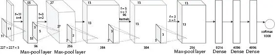
Figure 1.2 Architecture of AlexNet.
First Layer: AlexNet accepts a 227 × 227 × 3 RGB image as input which is fed to the first convolutional layer with 96 kernels (feature maps or filters) of size 11 × 11 × 3 and a stride of 4 and the dimension of the output image is changed to 96 images of size 55 × 55. The next layer is max-pooling layer or sub-sampling layer which uses a window size of 3 × 3 and a stride of two and produces an output image of size 27 × 27 × 96.
Second Layer: The second convolutional layer filters the 27 × 27 × 96 image with 256 kernels of size 5 × 5 and a stride of 1 pixel. Then, it is followed by max-pooling layer with filter size 3 × 3 and a stride of 2 and the output image is changed to 256 images of size 13 × 13.
Third, Fourth, and Fifth Layers: The third, fourth, and fifth convolutional layers uses filter size of 3 × 3 and a stride of one. The third and fourth convolutional layer has 384 feature maps, and fifth layer uses 256 filters. These layers are followed by a maximum pooling layer with filter size 3 × 3, a stride of 2 and have 256 feature maps.
Sixth Layer: The 6 × 6 × 256 image is flattened as a fully connected layer with 9,216 neurons (feature maps) of size 1 × 1.
Seventh and Eighth Layers: The seventh and eighth layers are fully connected layers with 4,096 neurons.
Output Layer: The activation used in the output layer is softmax and consists of 1,000 classes.
1.2.3 ZFNet
The architecture of ZFNet introduced by Zeiler [3] is same as that of the AlexNet, but convolutional layer uses reduced sized kernel 7 × 7 with stride 2. This reduction in the size will enable the network to obtain better hyper-parameters with less computational efficiency and helps to retain more features. The number of filters in the third, fourth and fifth convolutional layers are increased to 512, 1024, and 512. A new visualization technique, deconvolution (maps features to pixels), is used to analyze first and second layer’s feature map.
Table 1.3 AlexNet layer details.
| Sl. no. | Layer | Kernel size | Stride | Activation shape | Weights | Bias | # Parameters | Activation | # Connections |
| 1 | Input Layer | - | - | (227,227,3) | 0 | 0 | - | relu | - |
| 2 | CONV1 | 11 × 11 | 4 | (55,55,96) | 34,848 | 96 | 34,944 | relu | 105,415,200 |
| 3 | POOL1 | 3 × 3 | 2 | (27,27,96) | 0 | 0 | 0 | relu | - |
| 4 | CONV2 | 5 × 5 | 1 | (27,27,256) | 614,400 | 256 | 614,656 | relu | 111,974,400 |
| 5 | POOL2 | 3 × 3 | 2 | (13,13,256) | 0 | 0 | 0 | relu | - |
| 6 | CONV3 | 3 × 3 | 1 | (13,13,384) | 884,736 | 384 | 885,120 | relu | 149,520,384 |
| 7 | CONV4 | 3 × 3 | 1 | (13,13,384) | 1,327,104 | 384 | 1,327,488 | relu | 112,140,288 |
| 8 | CONV5 | 3 × 3 | 1 | (13,13,256) | 884,736 | 256 | 884,992 | relu | 74,760,192 |
| 9 | POOL3 | 3 × 3 | 2 | (6,6,256) | 0 | 0 | 0 | relu | - |
| 10 | FC | - | - | 9,216 | 37,748,736 | 4,096 | 37,752,832 | relu | 37,748,736 |
| 11 | FC | - | - | 4,096 | 16,777,216 | 4,096 | 16,781,312 | relu | 16,777,216 |
| 12 | FC | - | - | 4,096 | 4,096,000 | 1,000 | 4,097,000 | relu | 4,096,000 |
| OUTPUT | FC | - | - | 1,000 | - | - | 0 | softmax | - |
| - | - | - | - | - | - | - | 62,378,344 ( Total) | - | - |
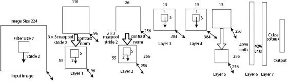
Figure 1.3 Architecture of ZFNet.
Читать дальшеИнтервал:
Закладка:
Похожие книги на «Computational Analysis and Deep Learning for Medical Care»
Представляем Вашему вниманию похожие книги на «Computational Analysis and Deep Learning for Medical Care» списком для выбора. Мы отобрали схожую по названию и смыслу литературу в надежде предоставить читателям больше вариантов отыскать новые, интересные, ещё непрочитанные произведения.


Обсуждение, отзывы о книге «Computational Analysis and Deep Learning for Medical Care» и просто собственные мнения читателей. Оставьте ваши комментарии, напишите, что Вы думаете о произведении, его смысле или главных героях. Укажите что конкретно понравилось, а что нет, и почему Вы так считаете.