Gene Cheung - Graph Spectral Image Processing

Vertex domain filtering may be typically defined as a local linear combination of the neighborhood samples

[1.9]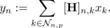

Since varies according to n , [ H] n,kshould be appropriately determined for all n . The matrix form of equation [1.9]may be represented as

[1.10]

where h ( W ) is a matrix containing filter coefficients h [ n, k ]( n k ) as a function of the adjacency matrix W, in which [ h ( W)] n,k= 0 if .

The vertex domain filtering in equations [1.9] and [1.10] requires the determination of filter coefficients, in general; moreover, it sometimes needs increased computational complexity. Typically, [ H] n,kmay be parameterized in the following form:

[1.11]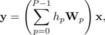

where h pis a real value and 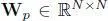is a masked adjacency matrix that only contains p- hop neighborhood elements of W. It is formulated as

[1.12]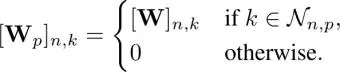

The number of parameters required in equation [1.12]is P , which is significantly smaller than that required in equation [1.10].

One may find a similarity between the time domain filtering in equation [1.2]and the parameterized vertex domain filtering in equation [1.11]. In fact, if the underlying graph is a cycle graph, equation [1.11]coincides with equation [1.2]with a proper definition of W p. However, they do not coincide in general cases: It is easily confirmed that the sum of each row of the filter coefficient matrix in equation [1.11]is not constant due to the irregular nature of the graph, whereas is a constant in time-domain filtering. Therefore, the parameters of equation [1.11]should be determined carefully.

The vertex domain filtering introduced above intuitively parallels time-domain filtering. However, it has a major drawback in a frequency perspective. As mentioned in section 1.2, time-domain filtering and frequency domain filtering are identical up to the DTFT. Unfortunately, in general, such a simple relationship does not hold in GSP. As a result, the naïve implementation of the vertex domain filtering equation [1.10]does not always have a diagonal response in the graph frequency domain. In other words, the filter coefficient matrix His not always diagonalizable by the GFT matrix U, i.e. U T HUis not diagonal in general. Therefore, the graph frequency response of His not always clear when filtering is performed in the vertex domain. This is a clear difference between the filtering of discrete-time signals and that of the graph signals.

From the above description, we can come up with another possibility for the filtering of graph signals: graph signal filtering defined in the graph frequency domain. This is an analog of filtering in the Fourier domain in equation [1.5]. This spectral domain definition of graph signal filtering has many desirable properties listed as follows:

– diagonal graph frequency response;

– fast computation;

– interpretability of pixel-dependent image filtering as graph spectral filtering.

These properties are described further.

As shown in equation [1.5], the convolution of h nand x nin the time domain is a multiplication of ĥ ( ω ) and in the Fourier domain. Filtering in the graph frequency domain utilizes such an analog to define generalized convolution (Shuman et al. 2016b):

[1.13]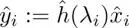

where 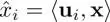is the i th GFT coefficient of xand the GFT basis u iis given by the eigendecomposition of the chosen graph operator equation [I.2]. Furthermore, is the graph frequency response of the graph filter. The filtered signal in the vertex domain, y [ n ], can be easily obtained by transforming ŷback to 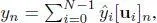where [ u i] nis the n th element of u i. This is equivalently written in the matrix form as

[1.14]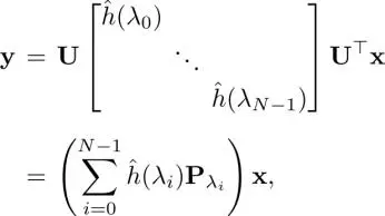

where

[1.15]

is a projection matrix in which σ ( λ ) is a set of indices for repeated eigenvalues, i.e. a set of indices such that Lu k = λ u k.

For simplicity, let us assume that all eigenvalues are distinct. Under a given GFT basis U, graph frequency domain filtering in equation [1.13]is realized by specifying N graph frequency responses in . Since this is a diagonal matrix, as shown in equation [1.14], its frequency characteristic becomes considerably clear in contrast to that observed in vertex domain filtering. Note that the naïve realization of equation [1.13]requires specific values of λ i, i.e. graph frequency values. Therefore, the eigenvalues of the graph operator must be given prior to the filtering. Instead, in this case, we can parameterize a continuous spectral response for the range λ ∈ [ λ min , λ max]. This graph-independent design procedure has been widely implemented in many spectral graph filters, since the eigenvalues often vary significantly in different graphs.