Gene Cheung - Graph Spectral Image Processing

Before we jump into the various chapters, we begin with the basic definitions in GSP that will be used throughout the book. Specifically, we formally define a graph, graph spectrum, variation operators and graph signal smoothness priors in the following sections.

A graph G ( V , E , W ) contains a set V of N nodes and a set E of M edges. While directed graphs are also possible, in this book we more commonly assume an undirected graph, where each existing edge ( i, j ) ∈ E is undirected and contains an edge weight w i,j ∈ R , which is typically positive. A large positive edge weight w i,jwould mean that samples at nodes i and j are expected to be similar/correlated.

There are many ways to compute appropriate edge weights. Especially common for images, edge weight w i,jcan be computed using a Gaussian kernel, as done in the bilateral filter (Tomasi and Manduchi 1998):

[I.1]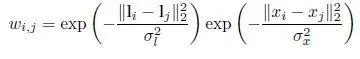

where l i ∈ R 2is the location of pixel i on the 2D image grid, x i ∈ R is the intensity of pixel i , and and are two parameters. Hence, 0 ≤ w i,j ≤ 1 . Larger geometric and/or photometric distances between pixels i and j would mean a smaller weight w i,j. Edge weights can alternatively be defined based on local pixel patches, features, etc. (Milanfar 2013b). To a large extent, the appropriate definition of edge weight is application dependent, as will be discussed in various forthcoming chapters.

A graph signal xon G is a discrete signal of dimension N – one sample x i ∈ R for each node 1 i in V . Assuming that nodes are appropriately labeled from 1 to N ,we can simply treat a graph signal as a vector x ∈ R N.

Denote by W ∈ R N×Nan adjacency matrix , where the ( i, j ) th entry is W i,j = w i,j. Next, denote by D ∈ R N×Na diagonal degree matrix , where the ( i, i ) th entry is D i,i = j W i,j. A combinatorial graph Laplacian matrix Lis L = D − W(Shuman et al . 2013). Because Lis real and symmetric, one can show, via the spectral theorem, that it can be eigen-decomposed into:

[I.2]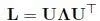

where Λis a diagonal matrix containing real eigenvalues λ kalong the diagonal, and Uis an eigen-matrix composed of orthogonal eigenvectors u ias columns. If all edge weights w i,jare restricted to be positive, then graph Laplacian Lcan be proven to be positive semi-definite (PSD) (Chung 1997) 2 , meaning that λ k ≥ 0 , ∀ k and x Lx ≥ 0 , ∀ x. Non-negative eigenvalues λ kcan be interpreted as graph frequencies , and eigenvectors Ucan be interpreted as corresponding graph Fourier modes. Together they define the graph spectrum for graph G .

The set of eigenvectors Ufor Lcollectively form the GFT (Shuman et al . 2013), which can be used to decompose a graph signal xinto its frequency components via α = U x. In fact, one can interpret GFT as a generalization of known discrete transforms like the Discrete Cosine Transform (DCT) (see Shuman et al . 2013 for details).

Note that if the multiplicity m kof an eigenvalue λ kis larger than 1, then the set of eigenvectors that span the corresponding eigen-subspace of dimension m kis non-unique. In this case, it is necessary to specify the graph spectrum as the collection of eigenvectors Uthemselves.

If we also consider negative edge weights w i,jthat reflect inter-pixel dissimilarity/anti-correlation, then graph Laplacian Lcan be indefinite. We will discuss a few recent works (Su et al. 2017; Cheung et al. 2018) that employ negative edges in later chapters.

Closely related to the combinatorial graph, Laplacian L, are other variants of Laplacian operators, each with their own unique spectral properties. A normalized graph Laplacian L n = D −1/2 LD −1/2is a symmetric normalized variant of L. In contrast, a random walk graph Laplacian L r = D −1 Lis an asymmetric normalized variant of L.A generalized graph Laplacian L g = L + diag ( D ) is a graph Laplacian with self-loops d i,iat nodes i – called the loopy graph Laplacian in Dörfler and Bullo (2013) – resulting in a general symmetric matrix with non-positive off-diagonal entries for a positive graph (Biyikoglu et al. 2005). Eigen-decomposition can also be performed on these operators to acquire a set of graph frequencies and graph Fourier modes. For example, normalized variants L nand L r(which are similarity transforms of each other) share the same eigenvalues between 0 and 2 . While Land L nare both symmetric, L ndoes not have the constant vector as an eigenvector. Asymmetric L rcan be symmetrized via left and right diagonal matrix multiplications (Milanfar 2013a). Different variation operators will be used throughout the book for different applications.

Traditionally, for graph G with positive edge weights, signal xis considered smooth if each sample x ion node i is similar to samples x jon neighboring nodes j with large w i,j. In the graph frequency domain, it means that xmostly contains low graph frequency components, i.e. coefficients α = U xare zeros (or mostly zeros) for high frequencies. The smoothest signal is the constant vector – the first eigenvector u 1for L, corresponding to the smallest eigenvalue λ 1 = 0 .