Gene Cheung - Graph Spectral Image Processing

Mathematically, we can declare that a signal xis smooth if its graph Laplacian regularizer (GLR) x Lxis small (Pang and Cheung 2017). GLR can be expressed as:

[I.3]

Because Lis PSD, x Lxis lower bounded by 0 and achieved when x = c u 1for some scalar constant c . One can also define GLR using the normalized graph Laplacian L ninstead of L, resulting in x L n x. The caveats is that the constant vector u 1– typically the most common signal in imaging – is no longer the first eigenvector, and thus .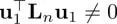

In Chen et al. (2015), the adjacency matrix Wis interpreted as a shift operator, and thus, graph signal smoothness is instead defined as the difference between a signal xand its shifted version Wx. Specifically, graph total variation (GTV) based on l p-norm is:

[I.4]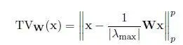

where λ maxis the eigenvalue of Wwith the largest magnitude (also called the spectral radius ), and p is a chosen integer. As a variant to equation [I.4], a quadratic smoothness prior is defined in Romano et al . (2017), using a row-stochastic version W n = D −1 Wof the adjacency matrix W:

[I.5]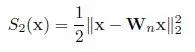

To avoid confusion, we will call equation [I.5]the graph shift variation (GSV) prior. GSV is easier to use in practice than GTV, since the computation of λ maxis required for GTV. Note that GSV, as defined in equation [I.5], can also be used for signals on directed graphs.

Biyikoglu, T., Leydold, J., Stadler, P.F. (2005). Nodal domain theorems and bipartite subgraphs. Electronic Journal of Linear Algebra , 13, 344–351.

Chen, S., Sandryhaila, A., Moura, J., Kovacevic, J. (2015). Signal recovery on graphs: Variation minimization. IEEE Transactions on Signal Processing , 63(17), 4609–4624.

Cheung, G., Su, W.-T., Mao, Y., Lin, C.-W. (2018). Robust semisupervised graph classifier learning with negative edge weights. IEEE Transactions on Signal and Information Processing over Networks , 4(4), 712–726.

Chung, F. (1997). Spectral graph theory. CBMS Regional Conference Series in Mathematics , 92.

Dörfler, F. and Bullo, F. (2013). Kron reduction of graphs with applications to electrical networks. IEEE Transactions on Circuits and Systems I: Regular Papers , 60(1), 150–163.

Lezoray, O. and Grady, L. (2012). Image Processing and Analysis with Graphs: Theory and Practice , CRC Press, Boca Raton, Florida.

Liu, X., Cheung, G., Wu, X., Zhao, D. (2017). Random walk graph Laplacian based smoothness prior for soft decoding of JPEG images. IEEE Transactions on Image Processing , 26(2), 509–524.

Milanfar, P. (2013a). Symmetrizing smoothing filters. SIAM Journal on Imaging Sciences , 6(1), 263–284.

Milanfar, P. (2013b). A tour of modern image filtering. IEEE Signal Processing Magazine , 30(1), 106–128.

Pang, J. and Cheung, G. (2017). Graph Laplacian regularization for image denoising: Analysis in the continuous domain. IEEE Transactions on Image Processing , 26(4), 1770–1785.

Romano, Y., Elad, M., Milanfar, P. (2017). The little engine that could: Regularization by denoising (RED). SIAM Journal on Imaging Sciences , 10(4), 1804–1844.

Shuman, D.I., Narang, S.K., Frossard, P., Ortega, A., Vandergheynst, P. (2013), The emerging field of signal processing on graphs: Extending high-dimensional data analysis to networks and other irregular domains. IEEE Signal Processing Magazine , 30(3), 83–98.

Su, W.-T., Cheung, G., Lin, C.-W. (2017). Graph Fourier transform with negative edges for depth image coding. IEEE International Conference on Image Processing , Beijing.

Tomasi, C. and Manduchi, R. (1998), Bilateral filtering for gray and color images. IEEE International Conference on Computer Vision , 839–846.

Vemulapalli, R., Tuzel, O., Liu, M.-Y. (2016). Deep Gaussian conditional random field network: A model-based deep network for discriminative denoising. Proceedings of the IEEE Conference on Computer Vision and Pattern Recognition , 4801–4809.

Zhang, K., Zuo, W., Chen, Y., Meng, D., Zhang, L. (2017). Beyond a Gaussian denoiser: Residual learning of deep CNN for image denoising. IEEE Transactions on Image Processing , 26(7), 3142–3155.

1 1If a graph node represents a pixel in an image, each pixel would typically have three color components: red, green and blue. For simplicity, one can treat each color component separately as a different graph signal.

2 2One can prove that a graph G with positive edge weights has PSD graph Laplacian L via the Gershgorin circle theorem: each Gershgorin disc corresponding to a row in L is located in the non-negative half-space, and since all eigenvalues reside inside the union of all discs, they are non-negative.

Yuichi TANAKA

Tokyo University of Agriculture and Technology, Japan

The filtering of time- and spatial-domain signals is one of the fundamental techniques for image processing and has been studied extensively to date. GSP can treat signals with irregular structures that are mathematically represented as graphs. Theories and methodologies for the filtering of graph signals are studied using spectral graph theory. In image processing, graphs are strong tools for representing structures formed by pixels, like edges and textures.

The filtering of graph signals is not only an extension of that for standard time- and spatial-domain signals, but it also has its own interesting properties. For example, GSP can represent traditional pixel-dependent image filtering methods as graph spectral domain filters. Furthermore, theory and design methods for wavelets and filter banks, which are studied extensively in signal and image processing, are also updated to treat graph signals.

In this chapter, the spectral-domain filtering of graph signals is introduced. In section 1.2, the filtering of time-domain signals is briefly described as a starting point. The filtering of graph signals, both in the vertex and spectral domains, is detailed in section 1.3, in addition to its relationship with classical filtering. Edge-preserving image smoothing is represented as a graph filter in section 1.4. Furthermore, a framework of filtering by multiple graph filters, i.e. graph wavelets and filter banks, is presented in section 1.5. Eventually, section 1.6introduces several fast computation methods of graph filtering. Finally, the concluding remarks of this chapter are discussed in section 1.7.