Gene Cheung - Graph Spectral Image Processing

where t > 0 is an arbitrary parameter that helps control the spreading speed caused by diffusion. Note that this method still needs eigendecomposition of the graph Laplacian if we decide to implement equation [1.21]naïvely. Instead, (Zhang and Hancock 2008) represent equation [1.21]using the Taylor series around the origin as follows:

[1.22]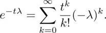

By truncating the above equation with an arbitrary order K , we can approximate the heat kernel as a finite-order polynomial (Hammond et al. 2011; Shuman et al . 2013). In Zhang and Hancock (2008), the Krylov subspace method is used, along with equation [1.22]to approximate the graph filter. The polynomial method for graph spectral smoothing is detailed in section 1.6.5.

Figure 1.2depicts the approximation error of the heat kernel using the Taylor series. Clearly, its approximation accuracy gets significantly worse when λ is away from 0. Since the maximum eigenvalue λ maxhighly depends on the graph used, it is better to use different approximation methods like the Chebyshev approximation, which is introduced in section 1.6.

Edge-preserving image smoothing is widely used for various tasks, as well as for image restoration (Nagao and Matsuyama 1979; Pomalaza-Raez and McGillem 1984; Weickert 1998; Tomasi and Manduchi 1998; Barash 2002; Durand and Dorsey 2002; Farbman et al. 2008; Xu et al. 2011; He et al . 2013). Image restoration aims to approximate an unknown ground-truth image from its degraded version(s). In contrast, edge-preserving smoothing is typically used to yield a user-desired image from the original one. The resulting image is not necessarily close to the original one.

In the graph setting, we need to define pixel-wise or patch-wise relationships as a distance between pixels or patches, and it is used to construct a graph. The following distances are often considered (Milanfar 2013b), where i and j are pixel or patch indices and is some nonnegative function:

1) Geometric distance: , where p iis the i th pixel coordinate.

2) Photometric distance: , where is the pixel value (often three dimensional) of the i th pixel/patch.

3) Saliency distance: 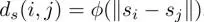where s iis the i th saliency value.

4) Combinations of the above.

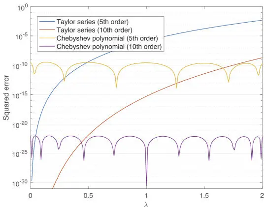
Figure 1.2. Comparison of approximation errors in . For a color version of this figure, see www.iste.co.uk/cheung/graph.zip

Saliency of the image/region/pixel is designed to simulate perceptual behavior (Itti et al. 1998; Harel et al. 2006). A popular choice of φ (·) is the Gaussian weight

[1.23]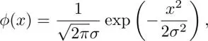

where σ controls the spread of the filter kernel.

Suppose that the filter coefficients are determined based on the above features, and that they are symmetric, i.e. the output pixel value y iis represented as

[1.24]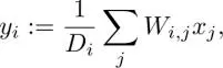

where

[1.25]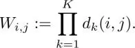

Here, d k(·, ·) is one of the distance metrics mentioned earlier and K is the number of features we considered. The scaling factor D inormalizes the filter weights as . For example, the bilateral filter is K = 2 for d g(·, ·) and d p(·, ·).

The Fourier domain representation of such pixel-dependent filters cannot be calculated in a classical sense because it is no longer shift-invariant: the filter matrix Wcannot be diagonalized by the DFT matrix. In contrast, GSP provides a frequency-like notion in the graph frequency domain. In general, the weight matrix Win equation [1.24]can be regarded as an adjacency matrix because all d k(·, ·) are assumed to be distances between pixels. Suppose that there is no self-loop in W, for simplicity. In general, the smoothed image in equation [1.24]is represented in the following matrix form:

[1.26]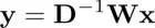

where D = diag( D 0 ,...,D N−1). This can be rewritten by using the relationship L= D− Was (Gadde et al . 2013):

[1.27]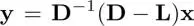

[1.28]

[1.29]

where is a degree-normalized signal. Let us denote the eigendecomposition of L nas . The above filtering in equation [1.29]is further rewritten as:

[1.30]

[1.31]

[1.32]