Gene Cheung - Graph Spectral Image Processing

Some precomputing methods have been proposed by Hu et al. (2015) and Zhang and Liang (2017), and they are mainly used for image compression. As expected, the GFT yields sparse transformed coefficients for piecewise smooth images/blocks. For those without such piecewise regions, conventional transforms like the DCT and DST are basically included as a set of precomputed bases.

To emphasize, the eigendecomposition of the graph operator will need complexity in general. In other words, we can reduce the complexity if we can assume graph signals on the underlying graph are bandlimited. Suppose that the signal is K- bandlimited, which is typically defined as

[1.50]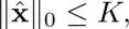

where ||·|| 0represents the number of non-zero elements, i.e. pseudo-norm. Here, without loss of generality, we can assume the first K GFT coefficients are non-zero:

[1.51]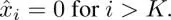

With the GFT basis U, it is equivalently represented as

[1.52]

where × represents some possible non-zero elements and

[1.53]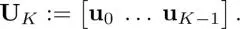

A partial eigendecomposition proposed in literature gives the following approximation of L:

[1.54]

Evaluating only requires K (< N ) eigenvectors and eigenvalues, which is significantly less than that obtained using the full eigendecomposition. In general, its computational complexity will be .

The previous subsection proposes that we can alleviate the heavy computational burden by assuming the bandlimitedness of the graph signal. However, this requires the assumption on the signal model prior to filtering, but the signal is not bandlimited in general.

In many application scenarios, we often only need the evaluation of xwith a given (linear) matrix function h ( L). That is, the eigenvalues and eigenvectors themselves are often unnecessary . The polynomial approximation methods introduced here enable us to calculate an approximation of y= h ( L) xwithout the (partial) decomposition of the variation operator.

Another advantage of filtering using a polynomial filter function is the vertex localization. The local filtering could capture local variations of pixel values, which are generally preferable. In contrast, filtering in the graph frequency domain ( equation [1.13]) is usually not localized in the vertex domain, because eigenvectors often have global support on the graph. Therefore, localizing graph filter response, both in the vertex and graph frequency domains, has been studied extensively (Shuman et al . 2013; Shuman et al. 2016b; Sakiyama et al. 2016). In fact, the localization of graph spectral filters can be controlled using polynomial filtering.

Polynomial graph filters are defined as follows:

[1.55]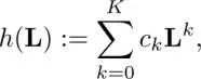

where c kis the k th order coefficient of the polynomial. It is known that each row of L kcollects its k- hop neighborhood; therefore, equation [1.55]is exactly the K- hop localized in the vertex domain. Note that L kcan be represented as

[1.56]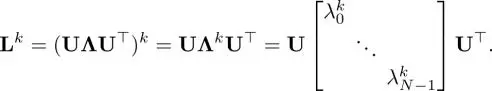

Here, we utilized the orthogonality of U. We can rewrite equation [1.55]by using equation [1.56]as:

[1.57]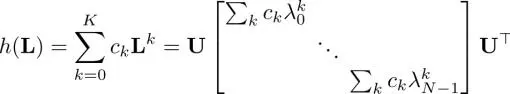

Consequently, the polynomial graph filter has the following graph frequency response:

[1.58]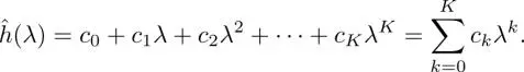

Especially, the output signal in the vertex domain is given by

[1.59]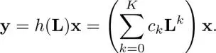

This indicates that we do not need to compute specific eigenvalues and eigenvectors for just calculating y. Specifically, we need to evaluate Lx, L 2 x ,..., L K x. Calculating Lz, where zis an arbitrary vector, requires complexity. Additionally, is required for computing c k L k x(and it is repeated K times). As a result, the entire complexity will be 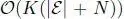. It is usually much lower than the partial eigendecomposition. In general, therefore, the number of edges is a dominant factor affecting the complexity.

Suppose that a fast computation is required for the spectral response of a graph filter , which is not a polynomial. Based on equation [1.59], we can approximate the output yif is satisfactorily approximated by a polynomial.

Any polynomial approximation methods, e.g. Taylor expansion, are possible for the above-mentioned polynomial filtering. In GSP, Chebyshev polynomial approximation is implemented frequently. The Chebyshev expansion gives an approximate minimax polynomial, i.e. the maximum approximation error can be reduced.