Ian Smith - Smith's Elements of Soil Mechanics
Здесь есть возможность читать онлайн «Ian Smith - Smith's Elements of Soil Mechanics» — ознакомительный отрывок электронной книги совершенно бесплатно, а после прочтения отрывка купить полную версию. В некоторых случаях можно слушать аудио, скачать через торрент в формате fb2 и присутствует краткое содержание. Жанр: unrecognised, на английском языке. Описание произведения, (предисловие) а так же отзывы посетителей доступны на портале библиотеки ЛибКат.

- Название:Smith's Elements of Soil Mechanics
- Автор:
- Жанр:
- Год:неизвестен
- ISBN:нет данных
- Рейтинг книги:5 / 5. Голосов: 1
-
Избранное:Добавить в избранное
- Отзывы:
-
Ваша оценка:
Smith's Elements of Soil Mechanics: краткое содержание, описание и аннотация
Предлагаем к чтению аннотацию, описание, краткое содержание или предисловие (зависит от того, что написал сам автор книги «Smith's Elements of Soil Mechanics»). Если вы не нашли необходимую информацию о книге — напишите в комментариях, мы постараемся отыскать её.
Smith's Elements of Soil Mechanics — читать онлайн ознакомительный отрывок
Ниже представлен текст книги, разбитый по страницам. Система сохранения места последней прочитанной страницы, позволяет с удобством читать онлайн бесплатно книгу «Smith's Elements of Soil Mechanics», без необходимости каждый раз заново искать на чём Вы остановились. Поставьте закладку, и сможете в любой момент перейти на страницу, на которой закончили чтение.
Интервал:
Закладка:
This graphical solution is only applicable to a dam resting on a permeable material. When the dam is sitting on impermeable soil, the phreatic surface cuts the downstream slope at a distance (a) up the slope from the toe ( Fig. 2.20a). The focus, F, is the toe of the dam, and the procedure is now to establish point C as before and draw the theoretical parabola ( Fig. 2.25a). This theoretical parabola will actually cut the downstream face at a distance Δa above the actual phreatic surface; Casagrande established a relationship between a and Δa in terms of α , the angle of the downstream slope ( Fig. 2.25b). In Fig. 2.25, the point J can thus be established, and the corrected flow line sketched in as shown.
Fig. 2.23 The parabola.
Fig. 2.24 Determination of upper flow line.
Fig. 2.25 Dam resting on an impermeable soil. (a) Construction for upper flow line. (b) Relationship between a and ∆a (after Casagrande).
2.15 Seepage through non‐uniform soil deposits
2.15.1 Stratification in compacted soils
Most loosely tipped deposits are probably isotropic, i.e. the value of permeability in the horizontal direction is the same as in the vertical direction. However, in the construction of embankments, spoil heaps, and dams, soil is placed and spread in loose layers which are then compacted. This construction technique results in a greater value of permeability in the horizontal direction, k x, than that in the vertical direction (the anisotropic condition). The value of k zis usually 1/5 to 1/10 the value of k x.
The general differential equation for flow was derived earlier in this chapter ( Equation 2.16):
For the two‐dimensional, i.e. anisotropic case, the equation becomes:
(2.28) 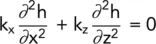
Unless k xis equal to k zthe equation is not a true Laplacian and cannot therefore be solved by a flow net. To obtain a graphical solution, the equation must be written in the form (i.e. divide through by k z):
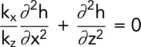
or
(2.29) 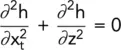
where

or

i.e.
(2.30) 
This equation is Laplacian and involves the two coordinate variables x tand z. It can be solved by a flow net provided that the net is drawn to a vertical scale of z and a horizontal scale of:
(2.31) 
2.15.2 Calculation of seepage quantities in an anisotropic soil
This is exactly as before:
(2.32) 
and the only problem is what value to use for k.
Using the transformed scale, a square flow net is drawn, and N fand N dare obtained. If we consider a ‘square’ in the transformed flow net, it will appear as shown in Fig. 2.26a. The same figure, drawn to natural scales (i.e. scale x = scale z), will appear as shown in Fig. 2.26b.
Let k ′ be the effective permeability for the anisotropic condition. Then k ′ is the operative permeability in Fig. 2.26a.
Hence, in Fig. 2.26a:
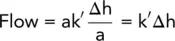
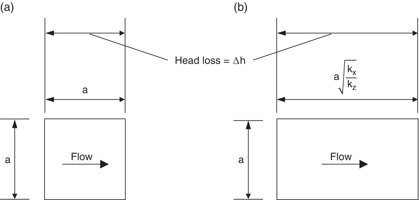
Fig. 2.26 Transformed and natural ‘squares’. (a) Transformed. (b) Natural.
and, in Fig. 2.26b:
(2.33) 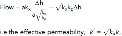
Example 2.8Seepage loss through dam (i)
The cross‐section of an earth dam is shown in Fig. 2.27a. Assuming that the water level remains constant at 35 m, determine the seepage loss through the dam. The width of the dam is 300 m, and the soil is isotropic with k = 5.8 × 10 −7m/s.
Solution:
The flow net is shown in Fig. 2.27b. From it, we have N f= 4.0 and N d= 14.
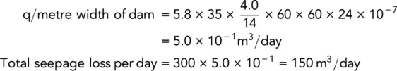
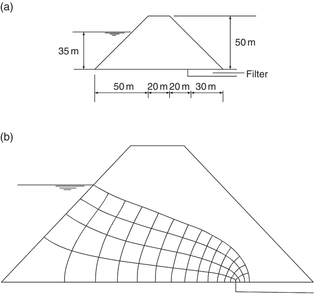
Fig. 2.27 Example 2.8. (a) The problem. (b) Flow net.
Example 2.9Seepage loss through dam (ii)
A dam has the same details as in Example 2.8except that the soil is anisotropic with k x= 5.8 × 10 −7m/s and k z= 2.3 × 10 −7m/s.
Determine the seepage loss through the dam.
Solution:
Transformed scale for x direction, 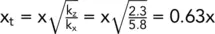
This means that, if the vertical scale is 1 : 500, then the horizontal scale is 0.63 : 500 or 1 : 794.
The flow net is shown in Fig. 2.28. From the flow net, N f= 5.0 and N d= 14.
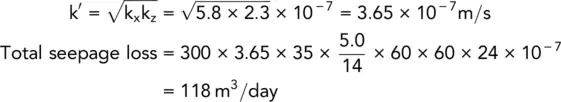
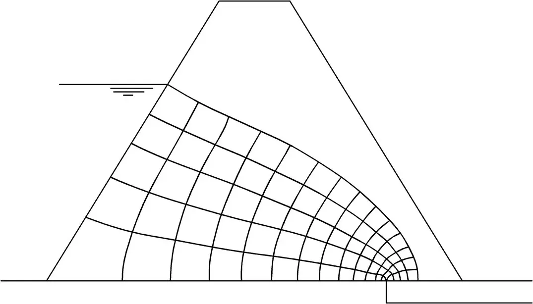
Fig. 2.28 Example 2.9.
Читать дальшеИнтервал:
Закладка:
Похожие книги на «Smith's Elements of Soil Mechanics»
Представляем Вашему вниманию похожие книги на «Smith's Elements of Soil Mechanics» списком для выбора. Мы отобрали схожую по названию и смыслу литературу в надежде предоставить читателям больше вариантов отыскать новые, интересные, ещё непрочитанные произведения.


Обсуждение, отзывы о книге «Smith's Elements of Soil Mechanics» и просто собственные мнения читателей. Оставьте ваши комментарии, напишите, что Вы думаете о произведении, его смысле или главных героях. Укажите что конкретно понравилось, а что нет, и почему Вы так считаете.