Ian Smith - Smith's Elements of Soil Mechanics
Здесь есть возможность читать онлайн «Ian Smith - Smith's Elements of Soil Mechanics» — ознакомительный отрывок электронной книги совершенно бесплатно, а после прочтения отрывка купить полную версию. В некоторых случаях можно слушать аудио, скачать через торрент в формате fb2 и присутствует краткое содержание. Жанр: unrecognised, на английском языке. Описание произведения, (предисловие) а так же отзывы посетителей доступны на портале библиотеки ЛибКат.

- Название:Smith's Elements of Soil Mechanics
- Автор:
- Жанр:
- Год:неизвестен
- ISBN:нет данных
- Рейтинг книги:5 / 5. Голосов: 1
-
Избранное:Добавить в избранное
- Отзывы:
-
Ваша оценка:
Smith's Elements of Soil Mechanics: краткое содержание, описание и аннотация
Предлагаем к чтению аннотацию, описание, краткое содержание или предисловие (зависит от того, что написал сам автор книги «Smith's Elements of Soil Mechanics»). Если вы не нашли необходимую информацию о книге — напишите в комментариях, мы постараемся отыскать её.
Smith's Elements of Soil Mechanics — читать онлайн ознакомительный отрывок
Ниже представлен текст книги, разбитый по страницам. Система сохранения места последней прочитанной страницы, позволяет с удобством читать онлайн бесплатно книгу «Smith's Elements of Soil Mechanics», без необходимости каждый раз заново искать на чём Вы остановились. Поставьте закладку, и сможете в любой момент перейти на страницу, на которой закончили чтение.
Интервал:
Закладка:
The flow of water through a soil can be represented graphically by a flow net ; a form of curvilinear net made up of a set of flow lines intersected by a set of equipotential lines .
Flow lines
The paths which water particles follow in the course of seepage are known as flow lines . Water flows from points of high to points of low head and makes smooth curves when changing direction. Hence, we can draw by hand or by computer, a series of smooth curves representing the paths followed by moving water particles.
Equipotential lines
As the water moves along the flow line, it experiences a continuous loss of head. If we can obtain the head causing flow at points along a flow line, then by joining up points of equal potential, we obtain a second set of lines known as equipotential lines .
2.10.1 Flow quantities
Referring back to Section 2.2.4, it is seen that the potential drop between two adjacent equipotentials divided by the distance between them is the hydraulic gradient. It attains a maximum along a path normal to the equipotentials and, in isotropic soil, the flow follows the paths of the steepest gradients so that flow lines cross equipotential lines at right angles.
Figure 2.8shows a typical flow net representing seepage through a soil beneath a dam. The flow is assumed to be two‐dimensional, a condition that covers a large number of seepage problems encountered in practice.
From Darcy's law q = Aki, so if we consider unit width of soil and if Δq = the unit flow through a flow channel (the space between adjacent flow lines), then:

where b = distance between the two flow lines.
In Fig. 2.8, the element ABCD is bounded by the same flow lines as element A 1B 1C 1D 1and by the same equipotentials as element A 2B 2C 2D 2.
For any element in the net, Δq = bki = bkΔh/l, where
Δh = head loss between the two equipotentials
l = distance between the equipotentials (see Fig. 2.9).
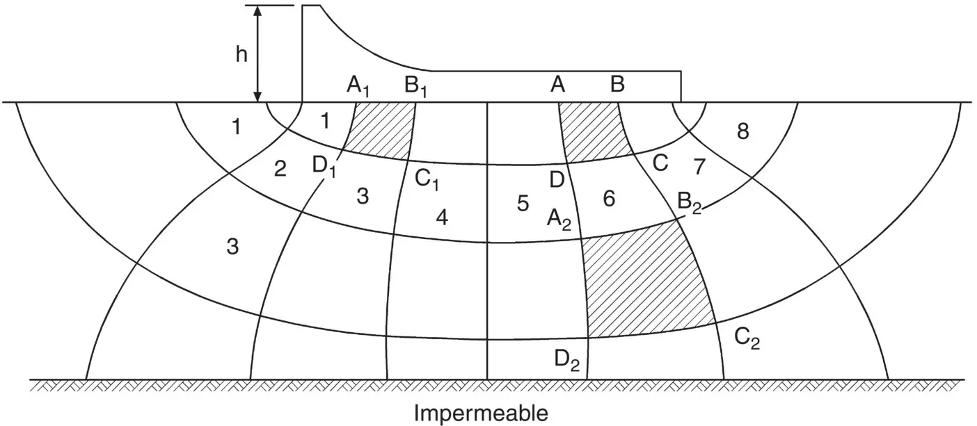
Fig. 2.8 Flow net for seepage beneath a dam.
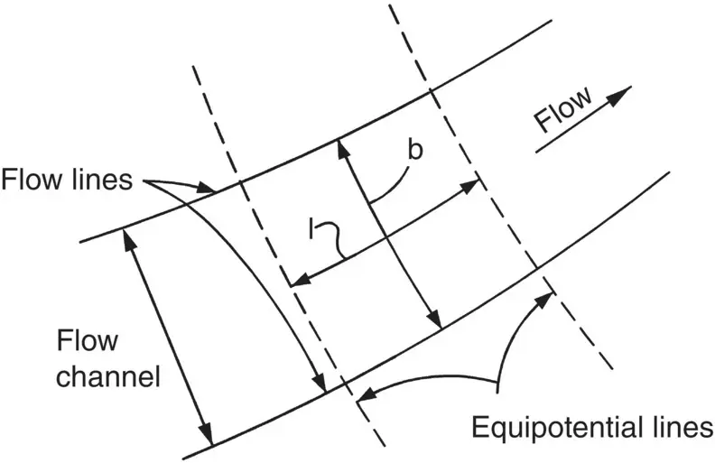
Fig. 2.9 Section of a flow net.
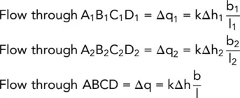
Referring to Fig. 2.8:
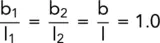
If we assume that the soil is homogeneous and isotropic then k is the same for all elements and it is possible to draw the flow net so that b 1= l 1, b 2= l 2, b = l. When we have this arrangement, the elements are termed ‘squares’ and the flow net is a square flow net. With this condition:
Since square ABCD has the same flow lines as A 1B 1C 1D 1,

Since square ABCD has the same equipotentials as A 2B 2C 2D 2,
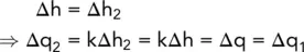
i.e.

Hence, in a flow net, where all the elements are square, there is the same quantity of unit flow through, and the same head drop across, each element.
No element in a flow net can be truly square, but the vast majority of the elements do approximate to squares in that the four corners of the element are at right angles and the distance between the flow lines, b, equals the distance between the equipotentials, l. Some relaxation is needed when asserting that a certain element is a square and some elements will be more triangular in shape but provided that the flow net is drawn with a sensible number of flow channels (generally five or six), the results obtained will be within the range of accuracy possible. The more flow channels that are drawn, the more the elements will approximate to true squares, but the apparent increase in accuracy is misleading and the extra work involved (if drawing by hand, for example, up to perhaps twelve channels) is not worthwhile.
2.10.2 Calculation of seepage quantities
Let
Nd = number of potential drops
Nf = number of flow channels
h = total head loss
q = total quantity of unit flow
Then
(2.21) 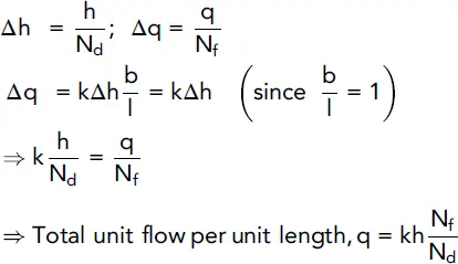
2.10.3 Drawing a flow net
The first step is to draw in pencil the first flow line, upon which the accuracy of the final correctness of the flow net depends. There are various boundary conditions that help to position this first flow line, including:
1 buried surfaces (e.g. the base of the dam, sheet piling), which are flow lines as water cannot penetrate into such surfaces;
2 the junction between a permeable and an impermeable material, which is also a flow line; for flow net purposes, a soil that has a permeability of one‐tenth or less the permeability of the other may be regarded as impermeable;
3 the horizontal ground surfaces on each side of the dam, which are equipotential lines.
The procedure is as follows:
1 draw the first flow line and hence establish the first flow channel;
2 divide the first flow channel into squares checking visually that b = l in each element;
3 project the equipotentials beyond the first flow channel, which gives an indication of the size of the squares in the next flow channel;
4 determine the position of the next flow line (remembering that b = l) draw this line as a smooth curve and complete the squares in the flow channel formed;
5 project the equipotentials and repeat the procedure until the flow net is completed.
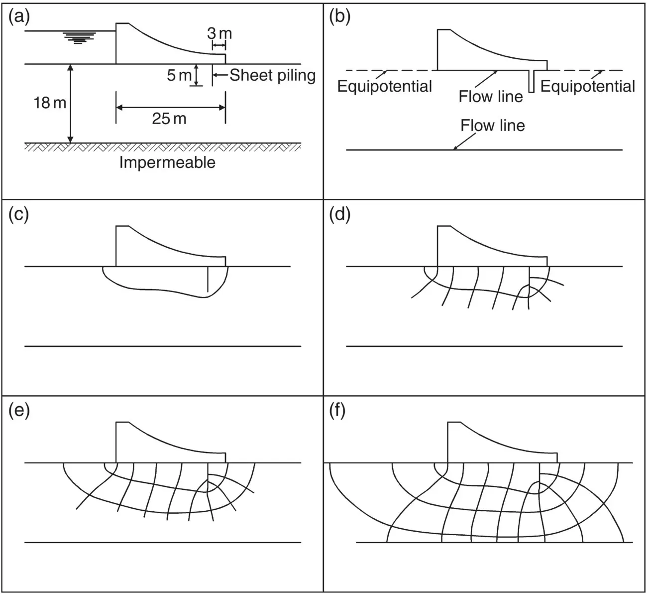
Fig. 2.10 Example of flow net construction. (a) Problem. (b) Boundary conditions. (c) Step a. (d) Step c. (e) Step d. (f) Final flow net.
As an example, suppose that it is necessary to draw the flow net for the conditions shown in Fig. 2.10a. The boundary conditions for this problem are shown in Fig. 2.10b, and the sketching procedure for the flow net is illustrated in figures c, d, e and f of Fig. 2.10.
If the flow net is correct, the following conditions will apply:
1 equipotentials will be at right angles to buried surfaces and the surface of the impermeable layer;
2 beneath the dam, the outermost flow line will be parallel to the surface of the impermeable layer.
Читать дальшеИнтервал:
Закладка:
Похожие книги на «Smith's Elements of Soil Mechanics»
Представляем Вашему вниманию похожие книги на «Smith's Elements of Soil Mechanics» списком для выбора. Мы отобрали схожую по названию и смыслу литературу в надежде предоставить читателям больше вариантов отыскать новые, интересные, ещё непрочитанные произведения.


Обсуждение, отзывы о книге «Smith's Elements of Soil Mechanics» и просто собственные мнения читателей. Оставьте ваши комментарии, напишите, что Вы думаете о произведении, его смысле или главных героях. Укажите что конкретно понравилось, а что нет, и почему Вы так считаете.