Yong Chen - Industrial Data Analytics for Diagnosis and Prognosis

mean(auto.spec.df$curb.weight) var(auto.spec.df$curb.weight) with(auto.spec.df, cov(curb.weight, length)) with(auto.spec.df, cor(curb.weight, length))> mean(auto.spec.df$curb.weight) [1] 2555.566 > var(auto.spec.df$curb.weight) [1] 271107.9 > with(auto.spec.df, cov(curb.weight, length)) [1] 5638.336 > with(auto.spec.df, cor(curb.weight, length)) [1] 0.8777285

Note the results above are somewhat different from those in Example 2.2because in this example we use the entire data set of auto.spec, instead of a small random subset of it as in Example 2.2.

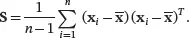
A multivariate data set consists of n observations collected from n items or units and each observation contains measurements on p variables, x 1, x 2,…, xp . The measurement vector for the i th observation is denoted by

The sample mean vector is the vector of sample means for the p variables, which is defined as

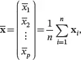
where x̄k is the sample mean of

The sample covariance matrix Sis the matrix of sample variances and covariances of the p variables:

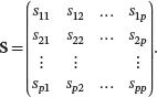
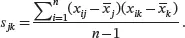
The off-diagonal elements of Sis the sample covariances of each pair of variables. For j ≠ k ,

(2.5)

The diagonal elements of S, sjj , j = 1,…, p are the sample variance of the j th variable. It is easy to see that when k = j , the sample covariance in ( 2.5) is equal to sj 2, the sample variance of the j th variable. So both notations sjj and sj 2represent the sample variance of xj . It is also obvious from ( 2.5) that skj . So the sample covariance matrix Sis a symmetric matrix. The sample covariance matrix Scan also be written by the observation vector x i as

(2.6)

Similarly, we define the sample correlation matrix as

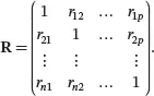
The ( j , k )th element of Ris the sample correlation of the j th and k th variables:

The sample correlation between a variable and itself is equal to 1. So the diagonal elements of a sample correlation matrix are all equal to 1. The sample correlation matrix Ris obviously symmetric since rjk = rkj .

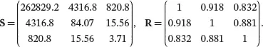
Example 2.4Consider the data set in Table 2.1. In Example 2.2, we found that x̄ 1= 2479.5 and x̄ 2= 170.35. Similarly, we can obtain x̄ 3= 65.41. So the mean vector of x= ( x 1 x 2 x 3) T is given by

In Example 2.2, we calculated the sample variances, sample covariance, and sample correlation of x 1and x 2. Similarly, we can obtain the sample variance of x 3and its sample covariance and correlation with the other two variables as

Note that while s 23is much smaller than s 13, r 23is greater than r 13, which indicates that the linear association between x 2and x 3is stronger than that of x 1and x 3. This clearly shows that the magnitude of the covariance itself is not meaningful in characterizing how strong the relationship of two variables is. Combining all the sample variance, covariance, and correlation information, the sample covariance matrix and sample correlation matrix of x= ( x 1 x 2 x 3) T can be written as

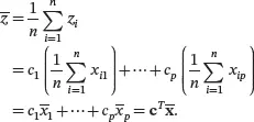
We are often interested in some linear combinations of the variables x 1, x 2,…, xp . For example, for the auto_specdata set, two of the variables are city.mpgand highway.mpg. If you expect that 60% of the mileage for a car is on highway and 40% is on local roads, then the average MPG for a car can be estimated as 0.6 × highway.mpg + 0.4 × city.mpg, which is a linear combination of city.mpgand highway.mpg. In general, let c 1, c 2,…, cp be constants and consider the linear combination of the variables x 1, x 2,…, xp given by

For each observation of the data set, the corresponding value of the variable z can be found by

where c T = ( c 1 c 2… cp ). It can be seen that the sample mean of z is

(2.7)

The sample variance of z can be found as

(2.8)

Because sample variance is always non-negative, for any c∈ ℛp we have c T Sc≥ 0 from ( 2.8). Therefore, the sample covariance matrix Sis always a positive semidefinite matrix.