Yong Chen - Industrial Data Analytics for Diagnosis and Prognosis

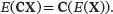
(3.1)

The covariance matrix of Z= CXis

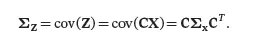(3.2)

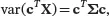
The similarity of ( 3.2) and (2.10) is pretty clear. When Cis a row vector c T= ( c 1, c 2,…, cp ), CX= c T X= c 1 X 1+ … + cp Xp and

(3.3)

(3.4)

where μand Σare the mean vector and covariance matrix of X.

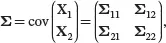
Let X 1and X 2denote two subvectors of X, i.e., . The mean vector and the covariance matrix of Xcan be partitioned as

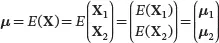(3.5)

(3.6)

where Σ 11= cov( X 1) and Σ 22= cov( X 2). The matrix Σ 12contains the covariance of each component in X 1and each component in X 2. Based on the symmetry of Σ, we have .

Normal distribution is the most commonly used distribution for continuous random variables. Many statistical models and inference methods are based on the univariate or multivariate normal distribution. One advantage of the normal distribution is its mathematical tractability. More importantly, the normal distribution turns out to be a good approximation to the “true” population distribution for many sample statistics and real-world data due to the central limit theorem , which says that the summation of a large number of independent observations from any population with the same mean and variance approximately follows a normal distribution.

Recall that a univariate random variable X with mean μ and variance σ 2is normally distributed, which is denoted by X ∼ N ( μ , σ 2), if it has the probability density function

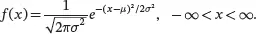(3.7)

The multivariate normal distribution is an extension of the univariate normal distribution. If a p -dimensional random vector Xfollows a multivariate normal distribution with mean vector μ and covariance matrix Σ, the probability density function of Xhas the form

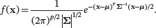(3.8)

We denote the p -dimensional normal distribution by Np ( μ , Σ).

From ( 3.8), the density of a p -dimensional normal distribution depends on xthrough the term ( x− μ ) T Σ −1( x− μ), which is the square of the distance from xto Σstandardized by the covariance matrix. Then it is clear that the set of xvalues yielding a constant height for the density form an ellipsoid. The set of points with the same height for the density is called a contour . The constant probability density contour of a p -dimensional normal distribution is:

which forms the surface of an ellipsoid centered at μwith standardized distance between xand μequal to c . And the contour with larger distance c has a smaller height value for the density. It can be shown that the axes of the ellipsoid contours of constant density for the p -dimensional normal distribution are in the directions of the eigenvectors of Σwith lengths proportional to the square roots of the corresponding eigenvalues of Σ.

Example 3.1:Consider a bivariate ( p = 2) normally distributed random vector X= ( X 1 X 2) T . Suppose the mean vector is μ = (0 0) T and the covariance matrix is

So the variance of both variables is equal to one and the covariance matrix coincides with the correlation matrix. The inverse of the covariance matrix is

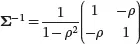
and | Σ| = 1 − ρ 2. Substituting Σ −1and | Σ| in ( 3.8), we have

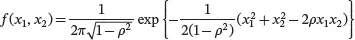(3.9)

From ( 3.9), if ρ = 0, the joint density can be written as f ( x 1, x 2) = f ( x 1) f ( x 2), where f ( x ) is the univariate normal density as given in ( 3.7), with μ = 0 and σ = 1. So in this case X 1and X 2are independent. This result is true for general multivariate normal distribution, as discussed later in this section.

By solving the characteristic equation | Σ− λ I| = 0, the two eigenvalues of Σare λ 1= 1 + ρ and λ 2= 1 – ρ . Based on Σv= λ v, the corresponding eigenvectors can be obtained as

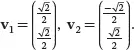
So the major axis of the ellipse contour of constant density is along the line x 1= x 2and the minor axis is orthogonal to the major axis. The larger the correlation coefficient ρ , the more elongated the ellipse contour. As an example, two bivariate normal distributions with ρ = 0 and ρ = 0.75 are shown in Figure 3.1(a) and Figure 3.1(b), respectively. Notice how the presence of correlation causes the probability distribution to concentrate along the line x 1= x 2. When ρ = 0, it is easy to see that the constant-density contour is a circle, as shown in Figure 3.2(a). For ρ = 0.75, the constant-density contour is an ellipse shown in Figure 3.2(b).