Fabio Giannino - Electromagnetic Methods in Geophysics
Здесь есть возможность читать онлайн «Fabio Giannino - Electromagnetic Methods in Geophysics» — ознакомительный отрывок электронной книги совершенно бесплатно, а после прочтения отрывка купить полную версию. В некоторых случаях можно слушать аудио, скачать через торрент в формате fb2 и присутствует краткое содержание. Жанр: unrecognised, на английском языке. Описание произведения, (предисловие) а так же отзывы посетителей доступны на портале библиотеки ЛибКат.
- Название:Electromagnetic Methods in Geophysics
- Автор:
- Жанр:
- Год:неизвестен
- ISBN:нет данных
- Рейтинг книги:4 / 5. Голосов: 1
-
Избранное:Добавить в избранное
- Отзывы:
-
Ваша оценка:
Electromagnetic Methods in Geophysics: краткое содержание, описание и аннотация
Предлагаем к чтению аннотацию, описание, краткое содержание или предисловие (зависит от того, что написал сам автор книги «Electromagnetic Methods in Geophysics»). Если вы не нашли необходимую информацию о книге — напишите в комментариях, мы постараемся отыскать её.
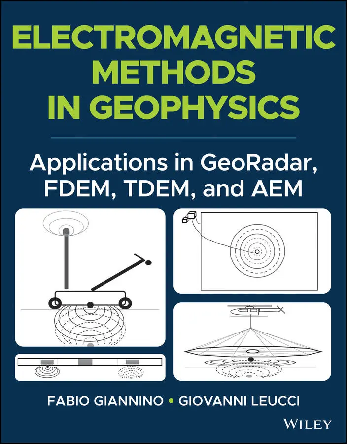
, accomplished researchers Fabio Giannino and Giovanni Leucci deliver an in-depth exploration of the theory and application of four different electromagnetic geophysical techniques: ground penetrating radar, the frequency domain electromagnetic method, the time domain electromagnetic method, and the airborne electromagnetic method. The authors offer a full description of each technique as they relate to the economics, planning, and logistics of deploying each of them on-site.
The book also discusses the potential output of each method and how it can be combined with other sources of below- and above-ground information to create a digitized common point cloud containing a wide variety of data.
Giannino and Leucci rely on 25 years of professional experience in over 40 countries around the world to provide readers with a fulsome description of the optimal use of GPR, FDEM, TDEM, and AEM, demonstrating their flexibility and applicability to a wide variety of use cases.
Readers will also benefit from the inclusion of:
A thorough introduction to electromagnetic theory, including the operative principles and theory of ground penetrating radar (GPR) and the frequency domain electromagnetic method (FDEM) An exploration of hardware architecture and surveying, including GPR, FDEM, time domain electromagnetic method (TDEM), and airborne electromagnetic (AEM) surveying A collection of case studies, including a multiple-geophysical archaeological GPR survey in Turkey and a UXO search in a building area in Italy using FDEM /li> Discussions of planning and mobilizing a campaign, the shipment and clearance of survey equipment, and managing the operative aspects of field activity Perfect for forensic and archaeological geophysicists,
will also earn a place in the libraries of anyone seeking a one-stop reference for the planning and deployment of GDR, FDEM, TDEM, and AEM surveying techniques.
Electromagnetic Methods in Geophysics — читать онлайн ознакомительный отрывок
Ниже представлен текст книги, разбитый по страницам. Система сохранения места последней прочитанной страницы, позволяет с удобством читать онлайн бесплатно книгу «Electromagnetic Methods in Geophysics», без необходимости каждый раз заново искать на чём Вы остановились. Поставьте закладку, и сможете в любой момент перейти на страницу, на которой закончили чтение.
Интервал:
Закладка:
In the EM helicopter borne systems (defined as HTEM), both the transmitting as well as the receiving loop, are carried below the helicopter in the same frame, at a height of about 30 to 40 meters above the ground level. In some systems, the receiver frame is independent from the transmitter frame.
AEM soundings are collected at approximately 1.5 seconds interval, which corresponds (taking into consideration the velocity of the helicopter) to a TDEM sounding (on land) approximately every 25 meters along the acquisition line. Actually, the sampling frequency may be defined during the post‐processing phase where a resampling can be performed with a finer stacking up to less than 5 meters.
The spacing between acquisition lines varies, from 50–100 meters to a few hundreds of meters, depending on the degree or resolution required and on the purpose of the survey.
AEM systems, may also host a GNSS, tilt meters, and altimeters used to control the position of the system, the inclination of the loops and the height from the ground, in continuous mode, allowing for the following correction during the data processing phase.
To summarize the phase of an AEM survey, starting from the data acquisition on the field to the data analyzed and visualized in office, the following can be concluded:
1 Once the most appropriate data acquisition system is selected based on the wave form emitted, and the survey is designed according to the purposes of the project, the data can be acquired on site.
2 EM data is visualized as Voltage variation in respect to time (along increasing time window). A first quality control is performed over each single 1D sounding, in order to verify that in no part of the survey area the data must be re‐collected because of a poor signal‐to‐noise ratio.
3 Then, each single 1D sounding is analyzed and filtered to enhance the quality of the signal, if needed. For each 1D signal a 1D inversion routine, is applied.
4 Finally, each single 1D model, is entered as input of a 2D or pseudo‐3D inversion routine to obtain 3D maps of the distribution of the resistivity.
Hereinafter, the principle and the basic equations related to the field quantities measured by AEM systems and the inversion will be presented.
As for the land FDEM and the TDEM method already presented, a transient magnetic field is generated by varying the flow of current around a transmitter loop. The EM field is thus generated, in order to diffuse downwards in the form of a plane wave. When the current abruptly interrupts the transmitter loop, this generates a variation in the magnetic field which induces an electromotive force ( emf ) in the medium (the half‐space below the ground encountered) according to Faraday’s Law of induction.
The magnitude emf is proportional to the rate of change of the primary magnetic field in the conductor. Hence, a current is induced in the conductor (the subsoil) like concentric horizontal eddy currents resembling smoke rings which run below the transmitter and diffuse through the medium (Nabighian, 1979).
As the time from the beginning of the primary generation passes, the induced current is weakened by the ground resistance and the current density increasingly weakens too. Therefore, currents decay over time (and depth for that matter). This phenomenon is, of course, a function of ground conductivity, and it occurs more slowly in highly conductive ground compared to poorly conductive ground (where currents diffuse and decay more quickly).
At this point, the secondary magnetic field generated by the induced currents and the rate of change of the secondary magnetic field, induces a voltage that is measured as a function of time that is sensed by an active receiver sensor (a receiving coil).
The uppermost layers have got a strong influence on the measured signal that is given in terms of nV/m2 at the receiver coil. As time passes and the current penetrates deeper into the ground, then the measured signal provides information on the conductivity of the lower layers, of course. And this is the way a receiver coil records information on the electrical conductivity as a function of depth. This type of information is, in fact, called the TEM sounding.
The period of time in which the transmitter is turned off is called ramp‐off . The on–off time is “designed” to emit signal at selected frequencies. The bandwidth of the system does not correlate directly with the system’s base frequency (which is the time window applied for collecting data), and it is largely determined by the frequency range of the primary EM field. The latter is not easy to establish, and to overcome this difficulty most TEM systems implement a linear shut‐off ramp for the current (Anderson, 1989).
The duration of the off‐ramp is inversely proportional to the high frequency bandwidth. A long linear ramp has the effect of making early time responses resemble a step response. A short linear ramp instead retains the characteristics of an impulse response (Palacky and West, 1991).
When deploying Airborne Transient EM systems these must be capable of handling the great variety of the earth’s responses with different ground conditions and they must cover very wide dynamic range to be effective. A good compromise between a rapid ramp off of the transmitter current and gradual shut off of the transmitter current represent a solution for resulting in early off‐time gates, which is appropriate for mapping near surface resistivity, on one side, and deeper ground penetration on the other. This is of course challenging to achieve at the same time and for one single configuration.
The timing at which the receiver coil TEM measurements are taken are quite narrow, and they are referred to as “time gates.” The early time gates are narrower than those at a late time because they occur when the transient voltage is changing rapidly. Also, at early time gates the SNR is higher and does not need a larger gate to be sampled as happens for late times. The early time gates thus provide information about the near surface, while late time gates provide information about the deeper subsoil.
The gates are spaced with a logarithmically increasing time period in order to minimize distortion of the transient voltage and improve the signal/noise (S/N) ratio at late times, a method called “log‐gating” (Siemon et al., 2009).
The mathematical expressions defining the components of the EM field are defined by the electromagnetic phenomena and are governed by Maxwell’s equations.
As already mentioned in Chapters 2.2 and 2.2 the relationships between electric field E, current J, and electric displacement D are described in two of these, while a second pair describe the relationships between magnetic field H, magnetic induction B, and magnetic polarization M. In quantitative terms, these four constitutive relations are:
(2.4.1) 
(2.4.2) 
(2.4.3) 
(2.4.4) 
where σ is electric conductivity, ε dielectric permittivity, μ magnetic permeability, and χ magnetic susceptibility.
The four parameters comprehensively describe the electromagnetic properties of a material. The first relation is effectively the well‐established Ohm’s law in a microscopic context. According to Maxwell’s laws, an alternating current induces secondary currents in a conductive earth. These secondary currents in turn generate secondary magnetic fields, measurable using EM receivers.
Читать дальшеИнтервал:
Закладка:
Похожие книги на «Electromagnetic Methods in Geophysics»
Представляем Вашему вниманию похожие книги на «Electromagnetic Methods in Geophysics» списком для выбора. Мы отобрали схожую по названию и смыслу литературу в надежде предоставить читателям больше вариантов отыскать новые, интересные, ещё непрочитанные произведения.


Обсуждение, отзывы о книге «Electromagnetic Methods in Geophysics» и просто собственные мнения читателей. Оставьте ваши комментарии, напишите, что Вы думаете о произведении, его смысле или главных героях. Укажите что конкретно понравилось, а что нет, и почему Вы так считаете.