Fabio Giannino - Electromagnetic Methods in Geophysics

From Figure 2.2.5it can be observed that a good conductor produces a strong Real component but a rather poor Imaginary component response (at high frequency), whereas an high‐resistive material (poor conductor), it produces a wide imaginary component, but a poor real component (low electrical conductivity and low frequency).

Let us consider a transmitting coil laying horizontally oriented with respect to the soil surface (vertical dipole mode), and a receiving coil, still in a vertical dipole mode, located at a (short) distance s from the transmitter coil, as sketched in figure 2.2.3.

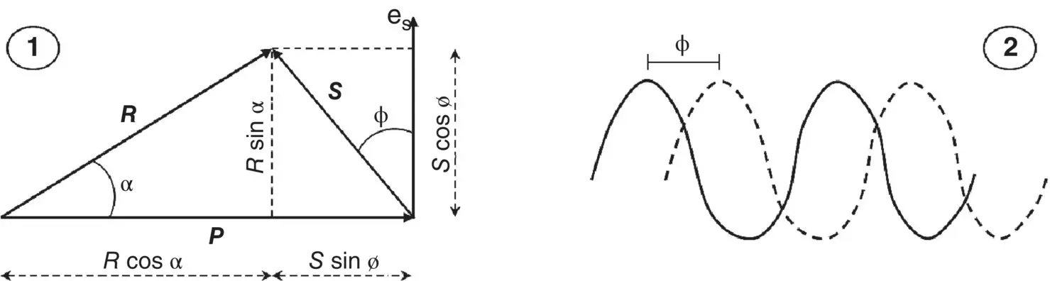
Figure 2.2.4 Sketch of the phase relation between the primary and the secondary EM field. 1) P is the primary, S the secondary and R represents the resulting EM field; e sis the EM induced field. 2) phase difference between two wave form

(modified from F. Giannino, 2014).

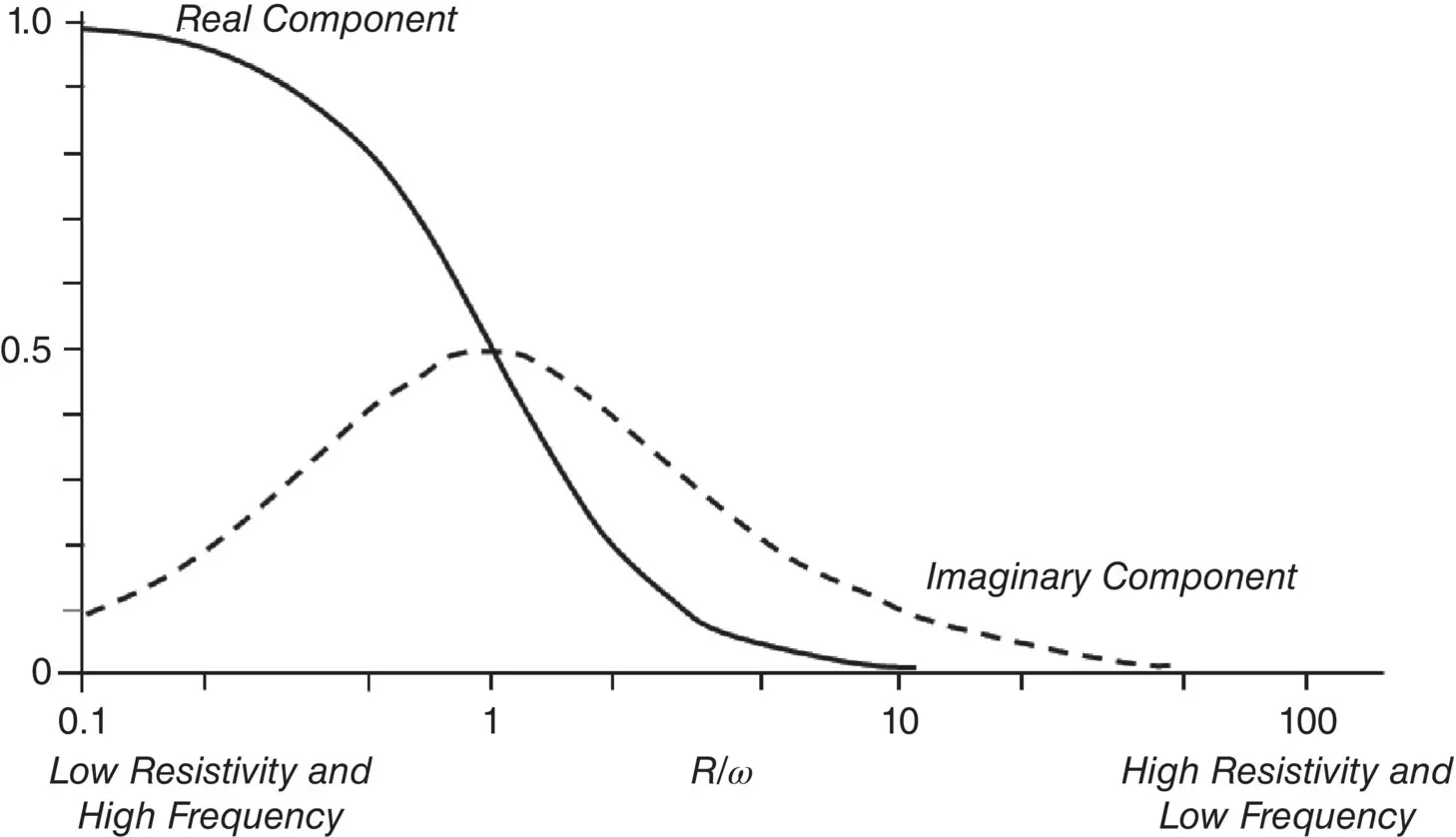
Figure 2.2.5 Sketch of the response of the Real component (solid line) and the Imaginary component (dashed line), as the ratio R/ω varies

(modified from F. Giannino, 2014).

When an alternating current flows within the transmitter coil, to this electric current is associated a magnetic field which, in turn, induces eddy current , in the subsoil; to the eddy currents , as in the case of the primary field, is associated a secondary magnetic field, that is sensed (detected) by the receiver coil, together with the primary magnetic field due to the primary electric field.

The secondary magnetic field, is a complex function of the transmitting and receiving coils spacing ( s ), of the transmitter frequency ( f ), and of the subsoil conductivity σ.

Under specific conditions, defined as operations at low induction number , it can be observed that the secondary magnetic field becomes a function of the above‐mentioned variables, easier to handle (J.D. McNeill, 1980, ASTM D6639‐01, 2008):

(2.2.12)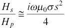

In 2.2.12, H sis the secondary magnetic field, H pis the primary magnetic field, ω is the angular frequency ( 2πf ), f is the frequency of the primary, μ 0is the magnetic permittivity in the free space, σ the electrical conductivity, s is the transmitting and receiving coil spacing, and .

As the above terms are either known or measured by any ground conductivity‐meter, it follows that the apparent electrical conductivity of the subsoil can easily be computed, via:

(2.2.13)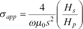

In order to have an explanation of the above, Figure 2.2.6should be considered.

In both cases shown in Figure 2.2.6(1 and 2), an alternating electric current of frequency f (in Hz), circulate within a transmitting coil, and the quantity actually measured at the receiver coil (Rx in Figure 2.2.6) is the ratio between the secondary and the primary magnetic field, hence H s/H p. The mathematical equations allowing for the computation of this ratio, either for the vertical dipole mode ( Figure 2.2.6– 1) as well as for the horizontal dipole mode ( Figure 2.2.6– 2), are:

(2.2.14)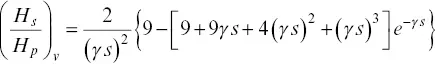

(2.2.15)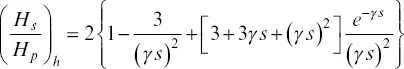

In (2.2.14), (vertical dipole mode) and 2.2.15, (horizontal dipole mode), s is the transmitting and receiving coil spacing, γ , ω=2πf , f is the frequency, μ 0is the magnetic permittivity in the free space, and .

Both (2.2.14)and (2.2.15), are rather complex functions of γs .

Under certain conditions, these two functions may be simplified, and they conduct back to the equation (2.2.13).

In order to explain the above (and to reach to the justification of the Low Induction Number conditions), let us consider one of the subsoil characteristics is the so‐called skin depth .

The skin depth is the distance from the EM source (depth) where the amplitude of a signal propagating through a homogeneous half‐space, reduces to 1/e with respect to the amplitude of the original signal emitted by the EM source itself.

The skin depth is denoted by δ , and can be written as:

(2.2.16)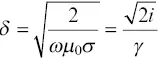

It follows that,

(2.2.17)

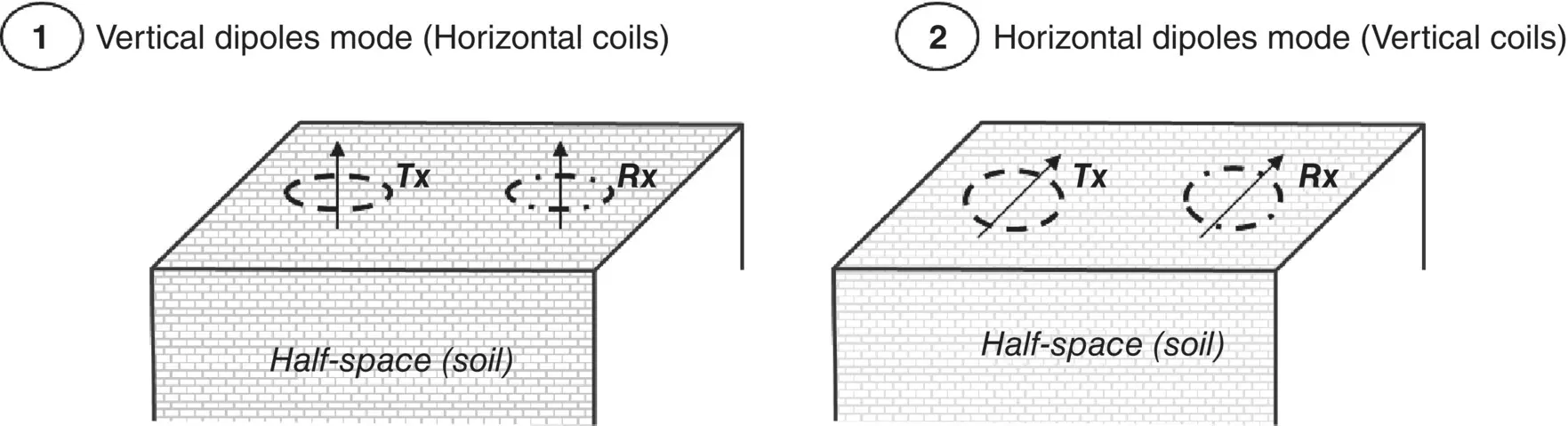
Figure 2.2.6 Vertical dipole (1) and horizontal dipole (2) FDEM data acquisition mode

(modified from J.D. McNeill, 1980).

In (3.2.17) the ratio is the so‐called induction numberand it is denoted by B : at condition that B is very small ( B <<1), and that the transmitting and receiving inter‐coil distance is very little with respect to the skin depth , (2.2.14)and (2.2.15)reduces to (3.2.13),

(2.2.18)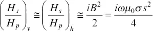

By resolving (3.2.18) with respect to σ, this brings back to 2.2.13,

A function that can be used alternatively for the computation of the skin depth is (P.V. Sharma, 1997):

(2.2.19)

Here ρ represents the electrical resistivity (Ω m), or the inverse of the electrical conductivity σ (σ =1/ ρ).

Under these operative conditions, that is when the inter‐coil spacing between the transmitter and the receiver is very small compared to the possible skin depth , the above approximation may be considered applicable and it facilitate the computation of the subsoil apparent conductivity.