Joseph Schmuller - Statistical Analysis with Excel For Dummies

If you select the first cell in the populated output array, the formula appears on the Formula bar in the usual way. If you select any other cell, the formula appears slightly grayer on the Formula bar.

On the iPad, you follow the same steps, but you complete some of them in a different way:

1 Enter the scores into an array of cells.No change. The numbers are in cells B2 through B16.

2 Enter the intervals into an array.Again, nothing different. The intervals are in C2 through C9.

3 Select a cell to start the output array.I tap cell D2.

4 From the Statistical Functions menu, select FREQUENCY to put the FREQUENCY formula into the Formula bar.This step highlights iPad's easier access to statistical functions. You just choose Formulas | Statistical and then select FREQUENCY. This step also shows the absence of dialog boxes from Excel on the iPad.

5 Use the formula in the Formula bar to enter the values of the arguments.In the Formula bar, the formula has the first argument, data_array, highlighted. (See Figure 2-11.) I select B2 through B16 to enter those cells into the formula's first argument.Next, I tap bins_array in the formula and select C2 through C9. If you find it difficult to select C2 and drag downward, select C9 and drag upward.

6 Press Return to put the values into the output array.

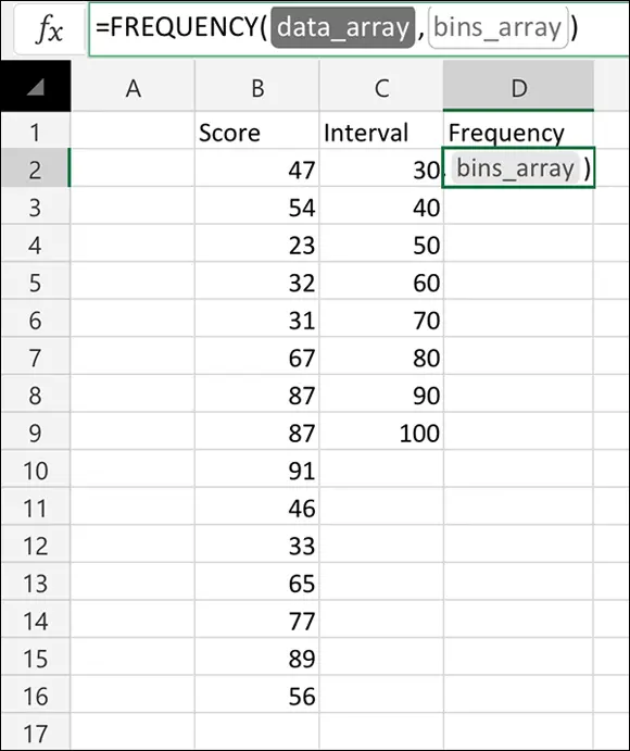
FIGURE 2-11:Working with FREQUENCYon the iPad.

As you get more into Excel’s statistical features, you work increasingly with formulas that have multiple arguments. Oftentimes, these arguments refer to arrays of cells, as in the examples I describe earlier in this chapter.

If you attach meaningful names to these arrays, it helps you keep straight what you’re doing. Also, if you return to a worksheet after not working on it for a while, meaningful array names can help you quickly get back into the swing of things. Another benefit: If you have to explain your worksheet and its formulas to others, meaningful array names are tremendously helpful.

Excel gives you an easy way to attach a name to a group of cells (but not on the iPad). In Figure 2-12, column C is named Revenue_Millions, indicating “revenue in millions of dollars.” As it stands, that just makes it a bit easier to read the column. If I explicitly tell Excel to treat Revenue_Millions as the name of the array of cells C2 through C13, however, I can use Revenue_Millions whenever I refer to that array of cells.

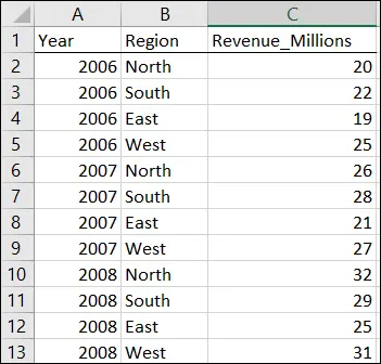
FIGURE 2-12:Defining names for arrays of cells.

Why did I use Revenue_Millions and not Revenue (Millions) or Revenue In Millions or Revenue: Millions? Because Excel doesn’t like blank spaces or symbols in its names — that’s why. In fact, here are four rules to follow when you supply a name for a range of cells. The name

Must begin with an alphabetic character — a letter rather than a number or a punctuation mark.

Must be unique within the workbook.

Cannot contain spaces or symbols (as I just mentioned) — use an underscore to denote a space between words in the name.

Cannot duplicate any cell reference in the worksheet.

Otherwise, Excel gives you up to 255 characters to get creative with the name.

Here’s how to define a name:

1 Add a descriptive name at the top of a column (or to the left of a row) you want to name.(Refer to Figure 2-10.)

2 Select the range of cells you want to name.In this example, that’s cells C2 through C13. Why not include C1? I explain in a second.

3 Right-click the selected range.This step opens the pop-up menu shown in Figure 2-13. FIGURE 2-13:Right-clicking a selected cell range opens this pop-up menu.

4 From this pop-up menu, choose Define Name.This selection opens the New Name dialog box. (See Figure 2-14.) As you can see, Excel knows that Revenue_Millions is the name of the array and that Revenue_Millions refers to cells C2 through C13. When presented with a selected range of cells to name, Excel looks for a nearby name — just above a column or just to the left of a row. If no name is present, you get to supply one in the New Name dialog box. (You can also open the New Name dialog box by choosing Formulas | Define Name.) FIGURE 2-14:The New Name dialog box. When you select a range of cells, like a column, with a name at the top, you can include the cell with the name in it and Excel attaches the name to the range. I strongly advise against doing this, however. Why? If I select C1 through C13, the name Revenue_Millions refers to cells C1 through C13, not C2 through C13. In that case, the first value in the range is text, and the others are numbers.For a formula such as SUM (or SUMIF or SUMIFS, which I discuss next), this doesn't make a difference: In those formulas, Excel just ignores values that aren’t numbers. If you have to use the whole array in a calculation, however, it makes a huge difference: Excel thinks the name is part of the array and tries to use it in the calculation. You see this in the next section, on creating your own array formulas.

5 Click OK.Excel attaches the name to the range of cells.

Now I have the convenience of using the name in a formula. Here, selecting a cell (like C14) and entering the SUMformula directly into C14 opens the boxes shown in Figure 2-15.

As the figure shows, the boxes open as you type. Selecting Revenue_Millions and pressing the Tab key fills in the formula in a way that Excel understands. You have to supply only the close parenthesis (see Figure 2-16) and press Enter in order to see the result.

Using the named array, then, the formula is

=SUM(Revenue_Millions)

which is more descriptive than

=SUM(C2:C13)

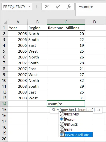
FIGURE 2-15:Entering a formula directly into a cell opens these boxes.

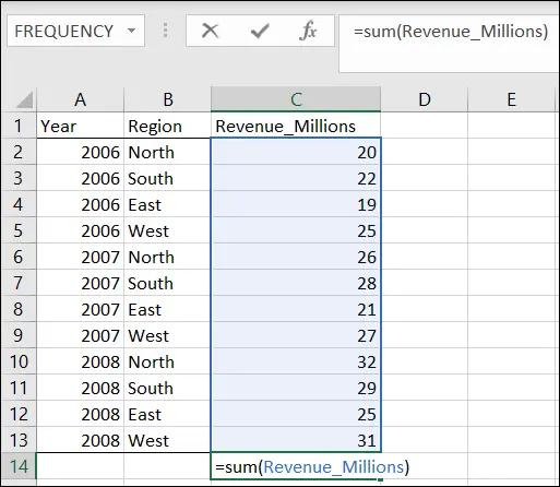
FIGURE 2-16:Completing the formula.

A couple of other formulas show just how convenient this naming capability can be. These formulas, SUMIFand SUMIFS, add a set of numbers if specific conditions in one cell range ( SUMIF) or in more than one cell range ( SUMIFS) are met.

To take full advantage of naming, I name my table's column A (Year) and column B (Region) in the same way I named column C.

When you define a name for a cell range like B2:B13 in this example, beware: Excel can be quirky when the cells hold names. It might guess that the name in the uppermost cell is the name you want to assign to the cell range. In this case, Excel guesses North for the name rather than Region. If that happens, you make the change in the New Name dialog box.

To keep track of the names in a worksheet, choose Formulas | Name Manager from the main menu to open the Name Manager box, shown in Figure 2-17. (The nearby buttons in the Defined Names area of the Ribbon — Define Name, Use in Formula, and Create from Selection — come in handy, so keep them in mind for the future.)