Joseph Schmuller - Statistical Analysis with Excel For Dummies

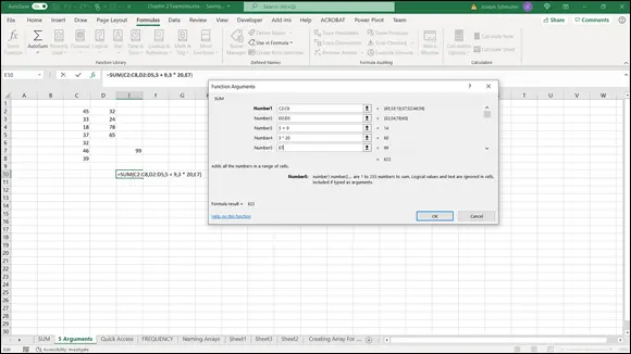
FIGURE 2-5:Using SUMwith five arguments.

If you select a cell in the same column as your data and just below the last data cell, Excel correctly guesses the data array you want to work on. Excel doesn't always guess what you want to do with that array, however. Sometimes when Excel does guess, its guess is incorrect. When either of those things happens, it’s up to you to enter the appropriate values into the Function Arguments dialog box.

In this section, I show you how to create a shortcut to Excel’s statistical functions.

You can get to Excel’s statistical functions by choosing Formulas | More Functions | Statistical and then choosing from the resulting pop-up menu. (See Figure 2-6.)

FIGURE 2-6:Accessing Excel’s statistical functions.

Although Excel has buried the statistical functions several layers deep, you can use a handy technique to make them as accessible as any of the other categories — just add them to the Quick Access toolbar in the upper left corner.

To do this, choose Formulas | More Functions from the main menu and then right-click the Statistical option. From the pop-up menu that appears, pick the first option, Add to Quick Access Toolbar. (See Figure 2-7.) Doing this adds a button to the Quick Access toolbar. Clicking the new button’s down arrow opens the pop-up menu of statistical functions. (See Figure 2-8.)

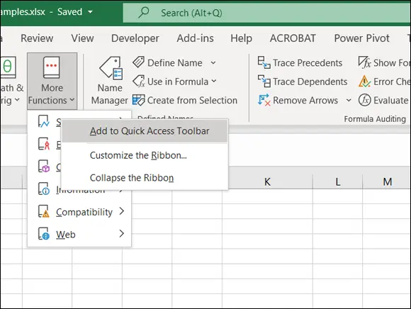
FIGURE 2-7:Adding the statistical functions to the Quick Access toolbar.

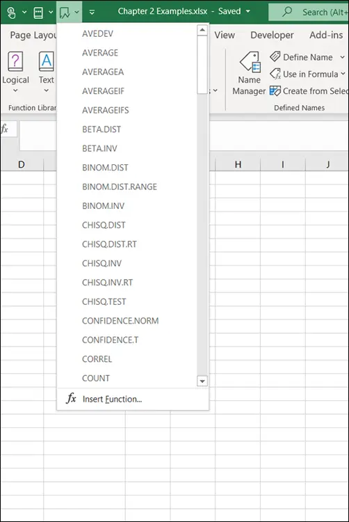
FIGURE 2-8:Accessing the Statistical Functions menu from the Quick Access toolbar.

Here’s how to put Statistical formulas into the Quick Access toolbar on the Mac. Choose Excel | Preferences | Ribbon & Toolbar and then click the Quick Access Toolbar tab. On the Choose Commands From menu, choose All Commands. Scroll down the box on the left, choose Statistical and click > to move Statistical to the box on the right. Click Save to put the Statistical icon into the Quick Access toolbar in the green area above the ribbon.

From now on, whenever I deal with a statistical function, I assume you’ve created this shortcut so that you can quickly open the menu of statistical functions. The next section provides an example.

On the iPad, no shortcut is necessary. To access statistical functions, it’s just Formulas | Statistical.

Remember that on the iPad the Statistical icon is to the immediate right of Math & Trig.

Most of Excel’s built-in functions are formulas that calculate a single value (like a sum) and put that value into a worksheet cell. Excel does have another type of function, however: It’s called an array function because it calculates multiple values and puts those values into an array of cells rather than into a single cell. I refer to this array as the output array .

This is where Microsoft 365 and Office 2019 part company. In Office 2019 and in earlier versions of Excel, here’s how you work with an array function: Select the range of cells, which will be the output array, open the array function’s dialog box, fill in the appropriate values, and then press the key combination Ctrl+Shift+Enter (or Ctrl+Shift+Return or Command+Shift+Return on the Mac) to close the dialog box and populate the output array. Readers of previous editions of this book might recall my frequent admonitions and warnings about that key combination whenever I talked about array functions. You can still select the output array and use the key combination in Microsoft 365, but it’s no longer necessary.

In Microsoft 365 (Windows, Mac, and iPad), you select only one cell, supply the appropriate information for the function, and just press Enter or click OK. Excel knows where the rest of the output array is and puts the computed values into its cells. It’s as if the computed values spilled over from the selected cell into the rest of the output array — so Microsoft refers to this process as spilling.

Throughout this book, I describe the Microsoft 365 procedure whenever I discuss an array function.

If you’re using Office 2019 (or an earlier version) of Excel, select the entire output array, supply the information that the function wants, and press Ctrl+Shift+Enter (Ctrl+Shift+Return or Command+Shift+Return on the Mac). I had to give you one last warning, for old times’ sake!

A good example of an array function is FREQUENCY(and it’s an Excel statistical function, too). Its job is to summarize a group of scores by showing how the scores fall into a set of intervals that you specify. For example, given the scores

77, 45, 44, 61, 52, 53, 68, 55

and the intervals

50, 60, 70, 80

FREQUENCYshows how many are less than or equal to 50 (2, in this example), how many are greater than 50 and less than or equal to 60 (that's 3), and so on. The number of scores in each interval is called a frequency. A table of the intervals and the frequencies is called a frequency distribution.

Here’s an example of how to use FREQUENCYin Microsoft 365:

1 Enter the scores into an array of cells.Figure 2-9 shows a group of scores in cells B2 through B16. FIGURE 2-9:Working with FREQUENCY.

2 Enter the intervals into an array.I’ve put the intervals in C2 through C9.

3 Select a cell to start the output array.I’ve put Frequency as the label in D1, so I select D2 to start the output array.

4 From the Statistical Functions menu, select FREQUENCY to open the Function Arguments dialog box.I use the shortcut I installed on the Quick Access toolbar to open this menu and select FREQUENCY.

5 In the Function Arguments dialog box, enter the appropriate values for the arguments.I begin with the Data_array box. In this box, I enter the cells that hold the scores. In this example, that's B2:B16. (I'm assuming you know Excel well enough to know how to do this in several ways.)Next, I identify the intervals array. FREQUENCY refers to intervals as bins and holds the intervals in the Bins_array box. In this example, C2:C9 goes into the Bins_array box. After I identify both arrays, the Insert Function dialog box shows the frequencies inside a pair of curly brackets: {}.

6 Click OK to close the Function Arguments dialog box and put the values in the output array.After you close the Function Arguments dialog box, the frequencies spill into the appropriate cells, as Figure 2-10 shows.

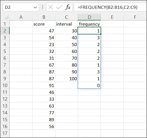
FIGURE 2-10:The finished frequencies.