Nirmal K. Sinha - Engineering Physics of High-Temperature Materials

Let us very briefly look at the essence of the technique of looking backward. The principle of the use of hindsight for a creep test is illustrated in Figure 1.4using the traditional presentation of linear timescale. In this case of a popular nickel‐base superalloy (Waspaloy), a tensile specimen is first loaded fully and rapidly (rise time <1 s) and unloaded completely (also in <1 s) after a creep time of 200 s, well within the transient or primary creep range, in comparison with 800 s for the time to reach the minimum creep rate for this level of stress. The axial strain recovery, after rapid removal of the load, was monitored for a relatively long time until a permanent or a viscous strain could be evaluated. Then, the same specimen was loaded for a long time to the accelerating tertiary stage and then fully unloaded, and strain recovery was recorded. For clarity, the strain level and time for the mcr for the longer‐term test are also shown. The mcr was determined from the strain rate versus time curve. The differences in the amount of permanent or viscous strain for the two tests are clearly noticeable. As expected, the permanent or viscous strain that occurred during the long test (duration of 2341 s) is significantly greater than that of the short test (for 200 s). Note the amount of elastic strain, delayed elastic strain, and viscous strain, shown for the longer‐term test. The delayed elastic strain is small, but not negligible. Similar observations were also noticed for the short‐time test. These observations provide clear indication that delayed elasticity, mostly ignored so far in high‐temperature rheological models emphasizing only mcr or steady‐state creep rate, should be given due consideration in order to get a better understanding of the mechanics of high‐temperature creep and failure. It should be mentioned here that the time span for full load application or the rise time of less than 1 s is also expected to minimize the scatter in the stress dependency of mcr as discussed by Bressers et al. (1981).

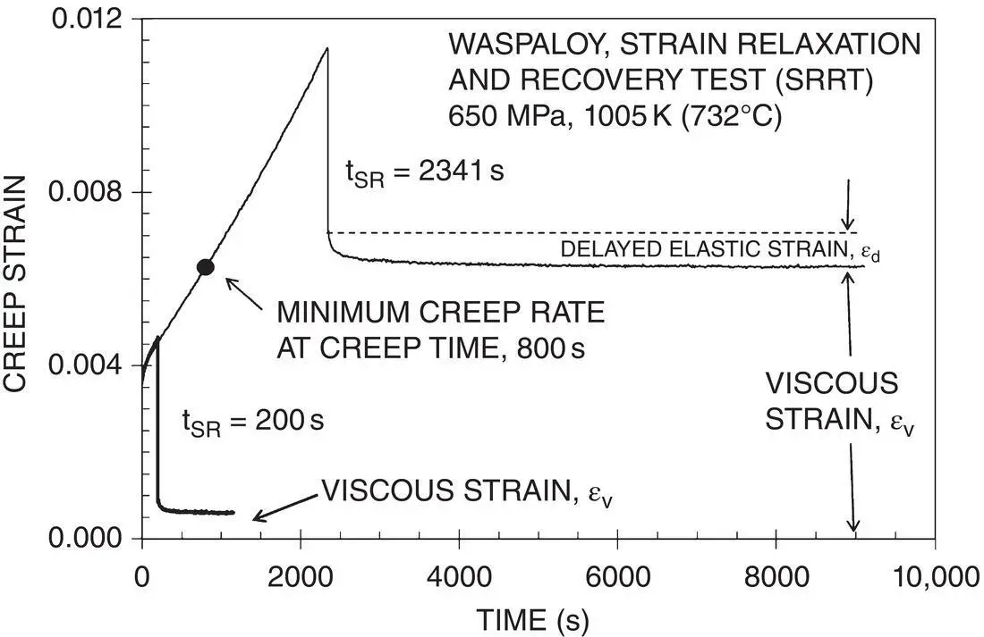
Figure 1.4 Short‐term (200 s) and longer‐term (2341 s) tensile SRRTs on a single specimen of polycrystalline nickel‐base superalloy Waspaloy at 1005 K (732 °C) for 650 MPa using linear timescale.

Source: N. K. Sinha.

There are innumerable sets of creep curves for a wide variety of manufactured and natural materials illustrating transient and tertiary creep stages, but the recovery on full unloading is rarely reported. There are, however, examples of stress‐dip tests in which creep continues after a short recovery on partial unloading during the steady state or actually at mcr that occurs at evolved microstructure corresponding to this state. Unfortunately, stress‐dip tests do not provide useful information on transient creep at the beginning of a creep test and the characteristics of neither the delayed elastic deformation nor the viscous flow corresponding to the original, undeformed and undamaged microstructure.

Figure 1.4exemplifies a unique set of results for a complex nickel‐based aerospace alloy. It brings out the fact that the delayed elastic strain, ε d, recovered on full unloading well within the tertiary stage of creep, after mcr, was not negligible and not “absorbed” within the viscous component. The long‐term test (2341 s) is noticeably larger than that of the 200 s test. Hence, ε dincreases with time. This raises the question as to the mechanism(s) responsible for generating delayed elasticity in polycrystalline materials that may have far‐reaching consequences, presented in Chapter 5, in developing physically based creep models.

Conventionally, a typical (often called normal) creep curve is described in terms of three stages: a primary regime during which the creep rate continuously decreases, a secondary regime where the creep rate is at a minimum, and a tertiary regime where the creep rate continuously increases, leading to rupture. All these three stages (except for the rupture) can be seen in the long‐term creep curve in Figure 1.5. The slope of the curve at a given time gives the creep rate at that time. It varies with time. However, the creep rate at a given time provides “total strain rate” or the rate of the “sum of reversible and irreversible strain” at that time. If the creep rate is plotted against time on a log–log scale, a typical creep response can be described by only two regimes: primary and tertiary. The minimum creep rate represents only the transition point between these two regimes. From the physics point of view, its numerical value provides no information either during the primary regime or the tertiary stage – the regimes important for engineering designs and life cycle management.

The use of the linear scale for time obscures the initial conditions of CL creep tests. Moreover, traditional methods of using a dead‐load lever system, although very simple and ideal for conducting very long‐term creep‐rupture tests with durations of 10 000 hours or more (e.g. Holdsworth et al. 2005; Yagi 2005; Kimura et al. 2009), do not allow the load to be applied as quickly as possible to satisfy the common assumption of “instantaneous” load application. Consequently, the materials science literature is full of the reported amount of initial strain on loading, ε ο. The use of linear timescale conveniently “hides” or obscures the weakness of the initial experimental conditions, albeit unavoidable for dead‐load systems. Nonetheless, a lot of undue emphasis has been put on the numerical values of ε ο. There is nothing fundamental about this initial strain. It simply depends on the test and data logging system and, to a greater degree, on the manual dexterity of an experimentalist. Figure 1.5presents the results of Figure 1.4using a logarithmic scale for time. Note the load‐application times of less than 1 s for both tests. This has been possible only by using a computer‐controlled closed‐loop servo‐hydraulic test system (described in Chapter 4).

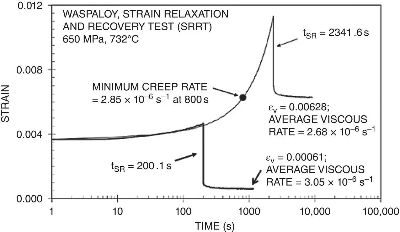
Figure 1.5 Results of Figure 1.4shown in a logarithmic timescale, illustrating load‐application times (<1 s) and similarities between the minimum creep rate of 2.85 × 10 −6s −1and the average viscous strain rates of 3.05 × 10 −6s −1and 2.68 × 10 −6s −1, respectively, for 200 s and 2432 s from the corresponding, ε v, at the end of recovery.

Source: N. K. Sinha.

Figure 1.5also shows the “average viscous strain rate”, , during the creep time or the “strain relaxation” time, t SR, of 200 s and 2432 s, respectively, given by

(1.1)

where ε vis the “measured permanent or viscous strain” after full recovery, as shown in Figure 1.5.

A set of five long‐term SRRT curves for Waspaloy is presented in Figure 1.6. All of these tests were carried out to periods well within the tertiary stages, but unloaded completely and extremely rapidly before fracturing and the strains were monitored for a long period to explore strain recoveries. Since the total strain even at unloading times was less than 1.2%, the true stress increased only slightly even at the time of unloading. These results are consistent with numerous published creep data in the literature, but with two important differences. These results present, for the first time to the authors’ knowledge, the systematic observations on creep recovery after full unloading during the tertiary stages and specimen response during “rise times” to apply the full load. Figure 1.6clearly illustrates the strain–time response during the “rise time” (from which elastic modulus E can be determined for each of the specimens). It also shows the creep curves with the corresponding minimum creep rates, and most importantly the permanent viscous strains, ε v, and the corresponding recovered delayed elastic strains, ε d(des), at the end of the tests. Analysis of the short‐term and long‐term SRRT data ( Figure 1.6) indicated that the creep strain at minimum creep rate consists of a significant amount of recoverable delayed elastic strain (32% at 450 MPa and 38% at 650 MPa).