Geophysical Monitoring for Geologic Carbon Storage

In an elastic Earth, the displacement at the surface, and in the overburden, is linearly related to the volume changes within the source region (Aki & Richards, 1980; Vasco et al., 1988). Thus, one can write the calculated displacements as an integral over with source volume V as

(2.7)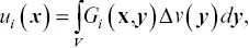

where Δ v ( y) is the fractional volume change at source location y. The quantity G i( x, y) is a Green's function representing the i ‐th displacement component at location x that results from a point volume increase at y. The Green's function encapsulates the physics of the propagation of elastic deformation from the source to the observation point, obtained by solving the governing equation with a point source. For a simple medium with sufficient symmetry, such as a homogeneous half‐space, it is possible to produce an analytic Green's function. For a more general medium, one must resort to numerical approaches in order to compute G i( x, y). Even a layered medium requires a numerical approach to compute the Green's function (Wang et al., 2006).

Equation (2.7)constitutes the forward problem whereby the injected volume is specified and the displacement at the observation points is calculated. For computational purposes, the source volume is usually decomposed into a discrete sum of N elementary volumes, such as rectangular grid blocks, and the total volume has the basis function representation

(2.8)

Note that the volumes may be taken to be quite small and sources are often decomposed into one or more point‐like sources. Substituting the volume expansion (2.8)into the integral 2.7, and using the linearity of integration, results in the expression

(2.9)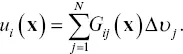

It is assumed that the fractional volume change given by Δυ iis constant over the elemental volume V j. The function G ij( x) represents the integral of the Green's function G i( x, y) over V j,

(2.10)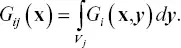

For InSAR observations, the data will consist of range‐change values, given by the projection of the displacement vector onto the satellite look vector l= ( l 1, l 2, l 3). Thus, the range change will be given by r = l⋅ uand the projection applied to equation 2.9gives

(2.11)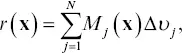

where the range change kernel M j( x) is

(2.12)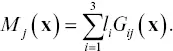

If we write the collective range‐change data for all of the pixels as a vector r, then the corresponding set of linear constraints, each in the form of equation 2.11, may be written as a matrix equation

(2.13)

In the inverse problem, observational data are used to estimate the distribution of volume change at depth. The most common approach is a least‐squares formulation in which one seeks a model v that minimizes the sum of the square of the residuals

(2.14)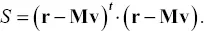

While it is possible to try to estimate the volume change for a full three‐dimensional source model by minimizing S , the solution will most likely be nonunique or poorly determined. That is, there will be many possible solutions and solving the least‐squares constraint equations will not lead to a stable answer. One can stabilize the solution by adding penalty terms to the misfit function S , representing aspects of the model that are considered undesirable, a procedure known as regularization . For example, the magnitude of deviations from an initial or prior model,

(2.15)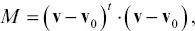

is often included as a penalty term. A term penalizing model roughness is also commonly used to regularize the inverse problem. Note that if one takes v 0equal to zero, the norm penalty will have the undesired effect of biasing the solution to have the largest changes at the shallowest depth. That is, in order to minimize the magnitude of the solution, most significant anomalies are placed close to the surface where they will have the greatest effect on the observations.

Given fluid injection and production data, it is often useful to constrain the changes in particular formations to try to honor the fluid volume information in addition to fitting the geodetic data. For example, given the net injected volumes, ν i, in a specific set of grid blocks, B I, we can add the penalty term

(2.16)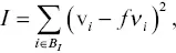

to the data misfit function S, where f is a scaling factor to account for the fact that the injection of a cubic meter of water leads to a change that is a fraction of the injected volume. If no such information is available, or if one is uncertain about how to scale the injected fluid volume to fractional volume changes at depth, it is still possible to penalize changes that are far from the well. That is, we can bias the solution to try to put the most significant volume changes near the injection site, where the pressure changes should be the largest. For example, if a well is located at x w, then the penalty function takes the form

(2.17)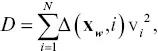

where Δ( x w, i ) is a function measuring the distance between the well and the center of the i ‐th grid block.

One of the advantages of geodetic observations is the relatively dense temporal sampling in comparison with other geophysical methods. For example, SAR data may be gathered at weekly to monthly intervals, leading to a time series of range change for each scatterer. Hence, it is possible to image the time evolution of the volume changes and to try and relate these changes to fluid movement and hydrological properties such as permeability (Vasco, 2004; Vasco et al., 2008; Rucci et al., 2010). The sequence of volume changes within each grid block of the reservoir model can be used to estimate an arrival or onset time, that moment at which the volume of a grid block is changing most rapidly. As discussed in Vasco et al. (2008), the onset time can be related to the travel time of the pressure front initiated by the start of injection. Specifically, for an elastic medium and a sharp injection profile resembling a step function, the onset of the peak rate of volume change, T peak, is related to the phase σ of the propagating pressure front according to (Vasco et al., 2000). For propagation governed by the diffusion equation, the phase is given by the solution of an eikonal equation,