Robert P. Dobrow - Probability
Здесь есть возможность читать онлайн «Robert P. Dobrow - Probability» — ознакомительный отрывок электронной книги совершенно бесплатно, а после прочтения отрывка купить полную версию. В некоторых случаях можно слушать аудио, скачать через торрент в формате fb2 и присутствует краткое содержание. Жанр: unrecognised, на английском языке. Описание произведения, (предисловие) а так же отзывы посетителей доступны на портале библиотеки ЛибКат.
- Название:Probability
- Автор:
- Жанр:
- Год:неизвестен
- ISBN:нет данных
- Рейтинг книги:4 / 5. Голосов: 1
-
Избранное:Добавить в избранное
- Отзывы:
-
Ваша оценка:
Probability: краткое содержание, описание и аннотация
Предлагаем к чтению аннотацию, описание, краткое содержание или предисловие (зависит от того, что написал сам автор книги «Probability»). Если вы не нашли необходимую информацию о книге — напишите в комментариях, мы постараемся отыскать её.
distinguished researchers Drs. Robert Dobrow and Amy Wagaman deliver a thorough introduction to the foundations of probability theory. The book includes a host of chapter exercises, examples in R with included code, and well-explained solutions. With new and improved discussions on reproducibility for random numbers and how to set seeds in R, and organizational changes, the new edition will be of use to anyone taking their first probability course within a mathematics, statistics, engineering, or data science program.
New exercises and supplemental materials support more engagement with R, and include new code samples to accompany examples in a variety of chapters and sections that didn’t include them in the first edition.
The new edition also includes for the first time:
A thorough discussion of reproducibility in the context of generating random numbers Revised sections and exercises on conditioning, and a renewed description of specifying PMFs and PDFs Substantial organizational changes to improve the flow of the material Additional descriptions and supplemental examples to the bivariate sections to assist students with a limited understanding of calculus Perfect for upper-level undergraduate students in a first course on probability theory, is also ideal for researchers seeking to learn probability from the ground up or those self-studying probability for the purpose of taking advanced coursework or preparing for actuarial exams.
Probability — читать онлайн ознакомительный отрывок
Ниже представлен текст книги, разбитый по страницам. Система сохранения места последней прочитанной страницы, позволяет с удобством читать онлайн бесплатно книгу «Probability», без необходимости каждый раз заново искать на чём Вы остановились. Поставьте закладку, и сможете в любой момент перейти на страницу, на которой закончили чтение.
Интервал:
Закладка:
The question was what are the chances that a Canfield solitaire laid out with 52 cards will come out successfully? After spending a lot of time trying to estimate them by pure combinatorial calculations, I wondered whether a more practical method than “abstract thinking” might not be to lay it out say one hundred times and simply observe and count the number of successful plays. This was already possible to envisage with the beginning of the new era of fast computers, and I immediately thought of problems of neutron diffusion and other questions of mathematical physics, and more generally how to change processes described by certain differential equations into an equivalent form interpretable as a succession of random operations. Later [in 1946], I described the idea to John von Neumann, and we began to plan actual calculations.
The Monte Carlo simulation approach is based on the relative frequency model for probabilities. Given a random experiment and some event  , the probability
  is estimated by repeating the random experiment many times and computing the proportion of times that
  occurs.
More formally, define a sequence  where
where
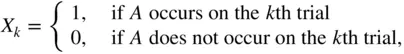
for  . Then
is the proportion of times in which  occurs in
  trials. For large
  , the Monte Carlo method estimates
  by
by
(1.7) 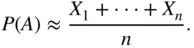
MONTE CARLO SIMULATION
Implementing a Monte Carlo simulation of  requires three steps:
1 Simulate a trial: Model, or translate, the random experiment using random numbers on the computer. One iteration of the experiment is called a “trial.”
2 Determine success: Based on the outcome of the trial, determine whether or not the event occurs. If yes, call that a “success.”
3 Replication: Repeat the aforementioned two steps many times. The proportion of successful trials is the simulated estimate of
Monte Carlo simulation is intuitive and matches up with our sense of how probabilities “should” behave. We give a theoretical justification for the method in Chapter 10, where we study limit theorems and the law of large numbers.
Here is a most simple, even trivial, starting example.
Example 1.32 Consider simulating the probability that an ideal fair coin comes up heads. One could do a physical simulation by just flipping a coin many times and taking the proportion of heads to estimate .Using a computer, choose the number of trials (the larger the better) and type the R command> sample(0:1, n, replace = T)The command samples with replacement from times such that outcomes are equally likely. Let 0 represent tails and 1 represent heads. The output is a sequence of ones and zeros corresponding to heads and tails. The average, or mean, of the list is precisely the proportion of ones. To simulate , type> mean(sample(0:1, n, replace = T))Repeat the command several times (use the up arrow key). These give repeated Monte Carlo estimates of the desired probability. Observe the accuracy in the estimate with one million trials:> mean(sample(0:1, 1000000, replace = T)) [1] 0.500376 > mean(sample(0:1, 1000000, replace = T)) [1] 0.499869 > mean(sample(0:1, 1000000, replace = T)) [1] 0.498946 > mean(sample(0:1, 1000000, replace = T)) [1] 0.500115
The Rscript CoinFlip.Rsimulates a familiar probability—the probability of getting three heads in three coin tosses.
R: SIMULATING THE PROBABILITY OF THREE HEADS IN THREE COIN TOSSES
# CoinFlip.R # Trial > trial <- sample(0:1, 3, replace = TRUE) # Success > if (sum(trial) == 3) 1 else 0 # Replication > n <- 10000 # Number of repetitions > simlist <- numeric(n) # Initialize vector > for (i in 1:n) { trial <- sample(0:1, 3, replace = TRUE) success <- if (sum(trial) == 3) 1 else 0 simlist[i] <- success } > mean(simlist) # Proportion of trials with 3 heads [1] 0.1293
The script is divided into three parts to illustrate (i) coding the trial, (ii) determining success, and (iii) implementing the replication.
To simulate three coin flips, use the samplecommand. Again letting 1 represent heads and 0 represent tails, the command
> trial <- sample(0:1, 3, replace = TRUE)
chooses a head or tails three times. The three results are stored as a three-element list (called a vector in R) in the variable trial.
After flipping three coins, the routine must decide whether or not they are all heads. This is done by summing the outcomes. The sum will equal three if and only if all flips are heads. This is checked with the command
> if (sum(trial) == 3) 1 else 0
which returns a 1 for success, and 0, otherwise.
For the actual simulation, the commands are repeated  times in a loop. The output from each trial is stored in the vector
 simlist. This vector will consist of  ones and zeros corresponding to success or failure for each trial, where success is flipping three heads.
Finally, after repeating  trials, we find the proportion of successes in all the trials, which is the proportion of ones in
 simlist. Given a list of zeros and ones, the average, or mean, of the list is precisely the proportion of ones in the list. The command mean(simlist)finds this average giving the simulated probability of getting three heads.
Run the script via the script file or Rsupplement to see that the resulting estimate is fairly close to the exact solution  Increase
  to 100,000 or even a million to get more precise estimates.
Интервал:
Закладка:
Похожие книги на «Probability»
Представляем Вашему вниманию похожие книги на «Probability» списком для выбора. Мы отобрали схожую по названию и смыслу литературу в надежде предоставить читателям больше вариантов отыскать новые, интересные, ещё непрочитанные произведения.


Обсуждение, отзывы о книге «Probability» и просто собственные мнения читателей. Оставьте ваши комментарии, напишите, что Вы думаете о произведении, его смысле или главных героях. Укажите что конкретно понравилось, а что нет, и почему Вы так считаете.