Mohammad H. Sadraey - Introduction to UAV Systems

The drag coefficient is the sum of two terms: (1) zero‐lift drag coefficient ( C Do) and (2) induced drag coefficient ( C Di). The first part is mainly a function of friction between air and the aircraft body (i.e., skin friction), but the second term is a function of local air pressure, which is represented by the lift coefficient. Pressure drag is mainly produced by flow separation. The sum of the pressure drag and skin friction (friction drag – primarily due to laminar flow) on a wing is called profile drag. This drag exists solely because of the viscosity of the fluid and the boundary layer phenomena.

The drag coefficient is a function of several parameters, particularly UAV configuration. A mathematical expression for the variation of the drag coefficient as a function of the lift coefficient is

(3.5)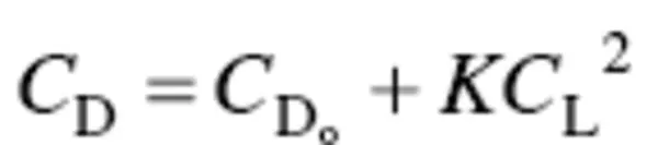

This equation is sometimes referred to as aircraft “drag polar.” The variable K is referred to as the induced drag correction factor. It is obtained from

(3.6)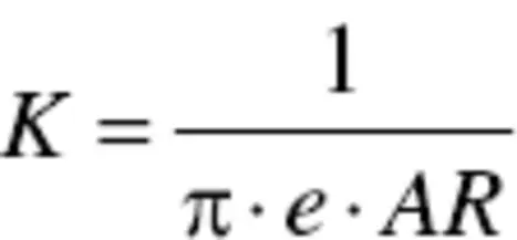

where e is the Oswald span efficiency factor and AR is the wing aspect ratio. The aspect ratio is defined as the ratio of wingspan over wing mean aerodynamic chord ( b / C ). It is also equal to wingspan squared divided by wing area or b 2 /S . The variable AR is further discussed in this chapter.

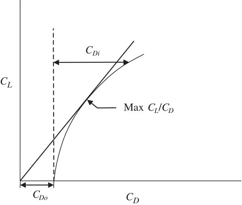
Figure 3.13 Airplane drag polar

A real three‐dimensional conventional aircraft normally is mainly composed of a wing, a fuselage, and a tail. The wing geometry has a shape, looking at it from the top, called the planform. It often has twist, sweepback, and dihedral (angle with the horizontal looking at it from the front) and is composed of two‐dimensional airfoil sections. The details of how to convert from the “infinite wing” coefficients to the coefficients of a real wing or of an entire aircraft is beyond the scope of this book, but the following discussion offers some insight into the things that must be considered in that conversion.

A full analysis for lift and drag must consider not only the contribution of the wing but also by the tail and fuselage and must account for varying airfoil cross‐section characteristics and twist along the span. Determining the three‐dimensional moment coefficient also is a complex procedure that must take into account the contributions from all parts of the aircraft.

A crude estimate (given without proof) of the three‐dimensional wing lift coefficient, indicated by an uppercase subscript ( C L), in terms of the “infinite wing” lift coefficient is

(3.7)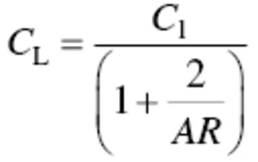

where C lis also the two‐dimensional airfoil lift coefficient. From this point onward, we will use uppercase subscripts, and assume that we are using coefficients that apply to the 3d wing and aircraft.

Drag of the three‐dimensional airplane wing plays a particularly important role in airplane design because of the influence of drag on performance and its relationship to the size and shape of the wing planform.

The most important element of drag introduced by a wing – at high angles of attack – is the “induced drag,” which is drag that is inseparably related to the lift provided by the wing. For this reason, the source of induced drag and the derivation of an equation that relates its magnitude to the lift of the wing will be described in some detail, although only in its simplest form.

The lowest induced drag is generated when the lift distribution over the wing is elliptical ( Figure 3.14), which provides a constant downwash along the span, as shown in Figure 3.14. Aerodynamicists in the past – including Ludwig Prandtl – believed that a wing whose planform is elliptical would have an elliptical lift distribution. But further research has not proven this idea. The notion of a constant downwash velocity ( w ) along the span will be the starting point for the development of the effect of three‐dimensional drag.

Considering the geometry of the flow with downwash, as shown in Figure 3.15, it can be seen that the downward velocity component for the airflow over the wing ( w ) results in a local “relative wind” flow that is deflected downward. This is shown at the bottom, where w is added to the velocity of the air mass passing over the wing ( V ) to determine the effective local relative wind ( V eff) over the wing. Therefore, the wing “sees” an angle of attack that is less than it would have had there been no downwash.

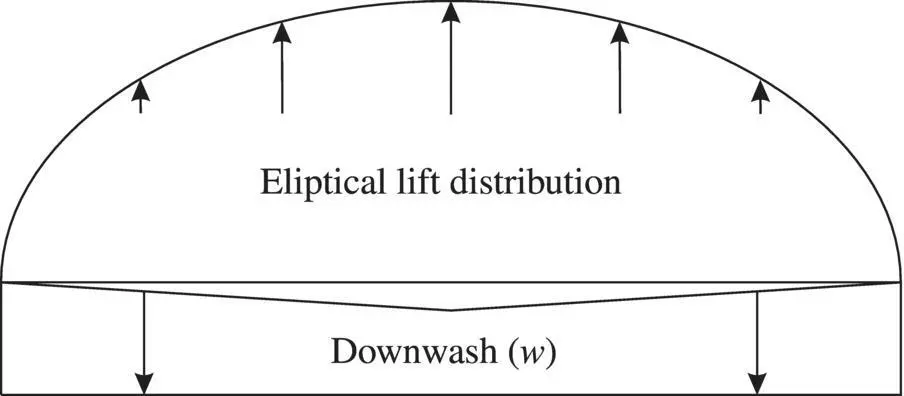
Figure 3.14 Elliptical lift distribution

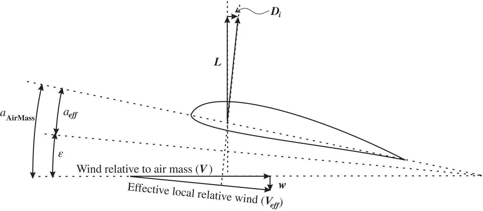
Figure 3.15 Induced drag diagram

The lift ( L ) is perpendicular to V and the net force on the wing is perpendicular to V eff. The difference between these two vectors, which is parallel to the velocity of the wing through the air mass, but opposed to it in direction, is the induced drag ( D i). This reduction in the angle of attack is

(3.8)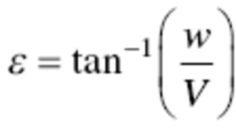

Then, the induced drag coefficient ( C Di) is given by

(3.9)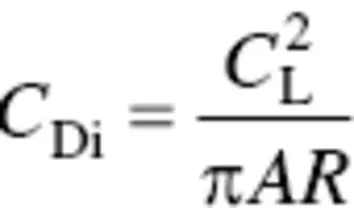

This expression reveals to us that air vehicles with short stubby wings (small AR ) will have relatively high‐induced drag and therefore suffer in range and endurance. Air vehicles that are required to stay aloft for long periods of time and/or have limited power, as, for instance, most electric‐motor‐driven UAVs, will have long (high AR) thin wings.

A fundamental axiom of fluid dynamics and aerodynamics is the notion that a fluid flowing over a surface has a very thin layer adjacent to the surface that sticks to it and therefore has a zero velocity. The next layer (or lamina) adjacent to the first has a very small velocity differential, relative to the first layer, whose magnitude depends on the viscosity of the fluid. The more viscous the fluid, the lower the velocity differential between each succeeding layer. At some distance δ , measured perpendicular to the surface, the velocity is equal to the free‐stream velocity of the fluid. The distance δ is defined as the thickness of the boundary layer (BL).