Magnetic Resonance Microscopy

(2.11)

The expression in Equation 2.11is valid with an accuracy around 2% or below in the following domain: [1]. A diversity of alternative simplified methods can be found in the literature, some extrapolated from experimental data [25,26], some using rough approximations about the boundary conditions at the dielectric interfaces [27] or implying the numerical solving of a transcendental equation [17], and others combining the above-mentioned approaches [21].

These estimation methods are valid for disk resonators, while the dielectric probe is described as a high-permittivity ( ϵ d= ϵ r ϵ 0) ring filled with a lower permittivity ( ϵ d= ϵ r,samp ϵ 0) sample. In the specific case of the TE 01δmode, equating the field distribution of the probe and the disk resonators is a reasonable approximation. Indeed, between the disk and the probe, the TE 01δmode features are affected in proportion to the electric and magnetic energies stored in the sample volume V samp[28]. The mode frequency varies from the value f diskfor the disk to f probefor the probe according to:

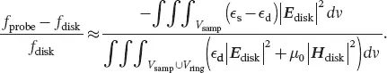(2.12)

As the region where the sample is located corresponds to the lowest values of the E-field distribution, the frequency shift due to the sample is limited. For the TE 01δmode, the ceramic probe is expected to be robust with respect to the sample loading while the permittivity contrast and the sample volume (or sample over disk radii ratio) have reasonable values. This is demonstrated in Figure 2.4.

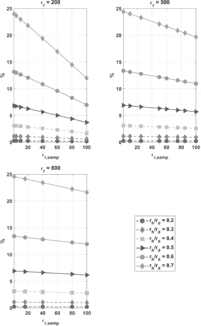
Figure 2.4 Quantification of the TE 01δmode frequency shift between the disk resonator and the dielectric probe (for both, the numerical simulations results were obtained with the CST Eigenmode Solver). The probe ring has its relative permittivity equal to 200, 500, and 800. The frequency variation is plotted as a function of the sample permittivity and for several discrete values of the radii ratio. Curves in dashed lines correspond to systematic frequency shift inferior to 5%. From [21].

One way of designing a ceramic probe as depicted in Figure 2.5 consists of studying how the achievable SNR varies with the probe dimensions and/or material properties for a given sample. In the following, the required field of view constrains the ring’s inner diameter and height, the ceramic material properties optimize the SNR value, and the outer diameter and the permittivity are used for tuning the resonance at the Larmor frequency. Therefore, designing the ceramic probe consists of the following steps:2.5

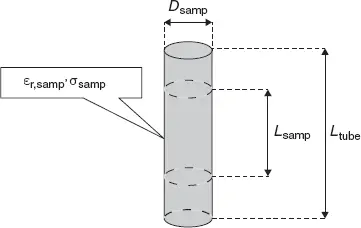
Figure 2.5 Schematics of the sample, typically contained in a water tube.

1 Define the required field of view: diameter Dsamp and length Lsamp. These two parameters define the inner radius of the dielectric ring rh, and its height L, respectively. The outer radius rd is kept as degree of freedom for tuning the mode at the Larmor frequency, and the material properties (permittivity ϵr and loss tangent tan δ) are used to optimize the achievable SNR.

2 For a given list of permittivity values estimate the required outer radii list for tuning at the Larmor frequency (Ne elements in each list).

Figure 2.6 is an example of such a tuning curve, with a target frequency of 730 MHz (Larmor frequency at 17 T), for a resonator with height 10 mm.

1 For a given list of loss tangent values (Nt values), estimate for each element of (and the associated outer radius for tuning) the corresponding SNR value (Ne × Nt values).

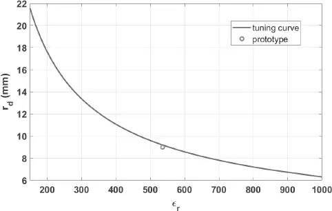
Figure 2.6 Example of tuning the first TE 01δmode frequency of a disk resonator with a given height through its outer radius for varying values of the permittivity.

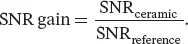
This array of SNR values can be used as it is for optimizing the ceramic properties, or divided by the corresponding SNR of another probe for comparison. In Figure 2.7, we display the SNR gain ( Equation 2.13) over a solenoid coil with the same inner dimensions loaded with the same sample, defined as follows:

On the left: as a function of the ceramic relative permittivity (vertical axis) and its loss tangent (horizontal axis) for given sample properties (ϵr,samp=50, σsamp = 1 S/m).

On the right: for the proposed prototype (ϵr = 536, tan δ = 8.10 −4) as a function of the sample relative permittivity and electrical conductivity.

(2.13)

Figure 2.7 Signal-to-noise ratio (SNR) gain displayed as a function of the ceramics properties for a given sample and fixed ring height and inner diameter (left) and of the sample properties for a fixed ceramic probe design (right). From [30].

With the abacus that can be drawn from such calculations it is possible to design a ceramic probe working under the first TE mode with optimized properties, and to predict the SNR enhancement compared to a reference probe.

The accuracy of this SNR estimation model and its constitutive steps was studied for ring resonators with dimensions fitting microscopic samples, and dielectric materials with permittivity adequate for the range of frequencies of MRM. For example, the normalized power loss term in Equation 2.8has been evaluated from the field distribution calculated in numerical simulations and with the semi-analytical method for varying electromagnetic properties of a sample for a given probe. As can be seen in Figure 2.8, the relative error between the two approaches never exceeds 5.1%. The SNR values predicted by numerical simulations and those obtained with the semi-analytical method are compared in Figure 2.9. The maximum relative error between the two approaches is 8% in the worst-case scenario.

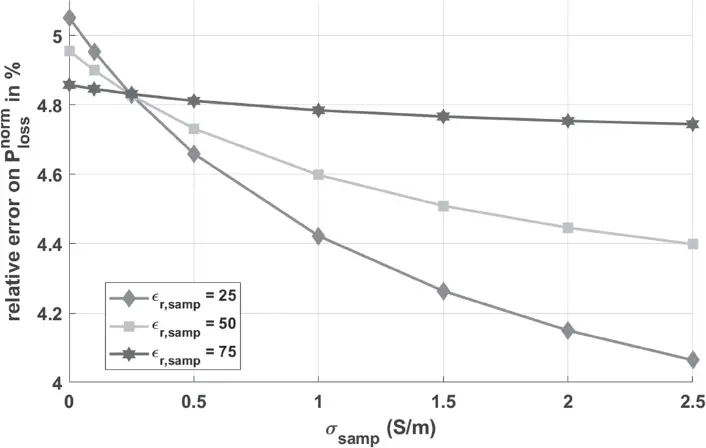
Figure 2.8 Relative error between the numerical simulations (CST Studio, Eigenmode Solver) and the semi-analytical model on the prediction of the normalized power losses term The error is plotted as a function of the sample conductivity and for three different sample permittivities. The ring resonator has the same properties as in [30]. The relative error is always below 5.1%. Figure reproduced with permission from [21].