Yang Xia - Essential Concepts in MRI

The time evolution of the Mz ( t ) component expressed by Eq. ( 2.29c) is illustrated in Figure 2.14e. Note that since T 1> T 2in most liquid-containing specimens, it takes much longer for Mz ( t ) to return to its thermal equilibrium than for My ( t ) and Mx ( t ) to decay to zero; that is, the time axes in the schematics in Figure 2.14 between (a) and (b) are scaled but between (a) and (e) or (b) and (e) are not scaled.

When a 90˚| y’ pulse is used in the excitation, the solutions of the Bloch equation take the form

(2.31a)

(2.31b)

(2.31c)

which only switches the oscillation terms between Mx ( t ) and My ( t ), or in other words the phase of the signal.

The frequency ω 0in Eq. (2.29) is usually too high for the voltage signal to be observed directly after amplification (a good linear amplifier at radio frequency is also more expensive). An electronic process named heterodyning is commonly used for signal detection in NMR. This process employs a number of phase-sensitive detectors to reduce the carrier frequency but retain the individual amplitude and phase information. This approach is identical to how we listen to a radio program – we do not really listen to our favorite broadcast program at hundreds of megahertz frequency (radio frequency); we listen to the audio frequency modulation of the radio broadcasting.

When Δ ω is used as the offset of the heterodyning signal, the NMR signal in the time domain, previously expressed in Eq. ( 2.30) in ω 0, becomes

(2.32)

where S 0is proportional to M 0, and ϕ is a spectrometer parameter called the receiver phase.

With the use of Fourier transformation, we can derive the signal in the frequency domain in both real (Re) and imaginary (Im) parts [2], as

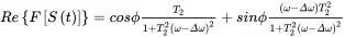(2.33a)

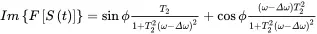(2.33b)

When ϕ = 0, the above equations become

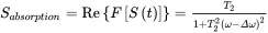(2.34a)

(2.34b)

These two equations can be plotted as in Figure 2.14c–d, where the real part is called the absorption signal, while the imaginary part is called the dispersion signal. By comparing Eq. (2.34) with Eq. (2.23) in the CW NMR experiment, we find that the results are of the same form as the absorption and dispersion components. However, the results in Eq. (2.34) are not centered at the Larmor frequency ω0 , but at the difference Δω , the offset frequency.

When ϕ ≠ 0, which is common in practice and means that Mis not along any axis in the transverse plane, the real and imaginary parts of the signal contain a mixture of absorption and dispersion components. We call the spectrum “out of phase.” We can correct this phase by multiplying the signal by exp(–i ϕ ); that is, we apply a 2D rotation matrix to the signal, as we did in Eq. ( 2.22). This process is termed to “phase” the spectrum in NMR experiments (cf. Chapter 6.10), which illustrates that in actual NMR experiments, the phase of the signal detector can be adjusted continuously.

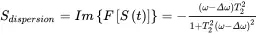
In classical physics, a variety of phenomena (e.g., the analysis of Hooke’s law in mechanics) can be characterized as simple harmonic motion, which is often visualized with the aid of a rotating disc. Plotting the trajectory of a fixed point on the rotating disc (or in the current context, the trajectory of the tip of a vector Min the 2D xy plane) as a function of time leads to a sinusoidal wave (Figure 2.15a and b). This type of circular motion can be described by a few fundamental equations,

Figure 2.15 (a) A vector Mrotates in the xy plane at a constant angular frequency ω and with a constant amplitude M , where the tip of the vector draws a sinusoidal wave in a plot of the amplitude vs. time, as in (b). (c) Four different initial orientations of the rotating vector give rise to four different phases of the wave, as shown in (d). The constant-amplitude oscillation implies no attenuation of the vector length. (e) When the oscillation is attenuated by an exponential decay, the motion of the rotating vector generates a damped oscillatory signal in the transverse plane (the FID). The FID signal will have the same decay envelope, regardless of which of the four initial orientations of the rotating vector shown in (c).

(2.35a)

(2.35b)

(2.35c)

where m is the amplitude of the motion, M is the maximum amplitude (i.e., the length of the vector), θ is the rotation angle in radian (rad), ω is the angular frequency in rad/s, T is the period of the wave (i.e., the time to complete one cycle) in seconds (s), and f is the frequency of the wave in hertz (Hz).

If no friction slows down the rotation of the disc and nothing changes the length of the vector, the disc will rotate at a constant frequency indefinitely and the wave will oscillate between +M and –M continuously as the function of time without any attenuation to its amplitude, as shown in Figure 2.15b. If the vector Min Figure 2.15a does not start the motion from being parallel with the x axis but with another axis, the oscillation will have exactly the same frequency and period, only with an extra phase shift (Figure 2.15c and d).

Similar visualization has in fact been used in the illustration of the motion of the magnetization in the laboratory and rotating frames (cf. Figure 1.3, Figure 2.14), except the FID signal has an attenuation term, which modulates the oscillation amplitude in the time domain. So instead of the constant amplitude sinusoidal waves as in Figure 2.15d, the amplitude of the FID oscillation will decay with time, as in Figure 2.15e, which generates the NMR signal. The only difference among the four NMR signals in Figure 2.15e is the four initial orientations of the magnetization vectors in the transverse plane (Figure 2.15c), that is, the initial phases of the magnetization. Even when Mdoes not start from being parallel with any axis in the transverse plane, the real and imaginary parts of the FID both start with some initial values but still oscillate and decay in the same manner as in Figure 2.15e.