Yang Xia - Essential Concepts in MRI
Здесь есть возможность читать онлайн «Yang Xia - Essential Concepts in MRI» — ознакомительный отрывок электронной книги совершенно бесплатно, а после прочтения отрывка купить полную версию. В некоторых случаях можно слушать аудио, скачать через торрент в формате fb2 и присутствует краткое содержание. Жанр: unrecognised, на английском языке. Описание произведения, (предисловие) а так же отзывы посетителей доступны на портале библиотеки ЛибКат.

- Название:Essential Concepts in MRI
- Автор:
- Жанр:
- Год:неизвестен
- ISBN:нет данных
- Рейтинг книги:5 / 5. Голосов: 1
-
Избранное:Добавить в избранное
- Отзывы:
-
Ваша оценка:
Essential Concepts in MRI: краткое содержание, описание и аннотация
Предлагаем к чтению аннотацию, описание, краткое содержание или предисловие (зависит от того, что написал сам автор книги «Essential Concepts in MRI»). Если вы не нашли необходимую информацию о книге — напишите в комментариях, мы постараемся отыскать её.
A concise and complete introductory treatment of NMR and MRI Essential Concepts in MRI
Essential Concepts in MRI
Essential Concepts in MRI — читать онлайн ознакомительный отрывок
Ниже представлен текст книги, разбитый по страницам. Система сохранения места последней прочитанной страницы, позволяет с удобством читать онлайн бесплатно книгу «Essential Concepts in MRI», без необходимости каждый раз заново искать на чём Вы остановились. Поставьте закладку, и сможете в любой момент перейти на страницу, на которой закончили чтение.
Интервал:
Закладка:
 (2.17)
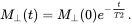
The motion of magnetization in spin-spin relaxation is shown schematically in Figure 2.10, where again t = 0 marks the moment that the B 1field is turned off.
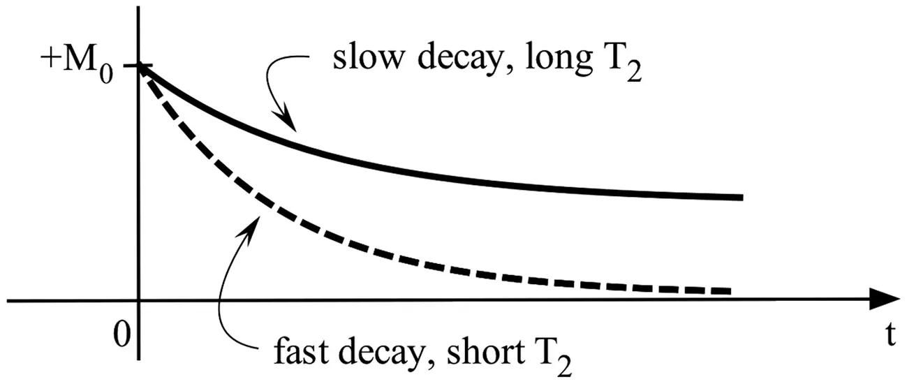
Figure 2.10 The motion of the magnitude of the transverse magnetization after a 90˚ B 1field/pulse, where a slow decay leads to a long T 2value. Note that if Figure 2.9 and Figure 2.10 are plotted together on one graph (i.e., share the same scale in the horizontal axis t ), the transverse magnetization would decay to zero much faster than the return of the longitudinal magnetization to its thermal equilibrium (i.e., the maximum), since T 2is commonly much shorter than T 1.
The decay of a time-domain signal in the transverse plane leads to a spectral broadening in the frequency domain (cf. Section 2.8 and Appendix A1.2 for Fourier transform). The line broadening due to the relaxation processes is named homogeneous and is inherently irreversible. In practice, the signal decays faster than the intrinsic rate due to the T 2relaxation. Other contributions to the signal decay include, for example, the inhomogeneity of the magnetic field B 0or low-frequency molecular motions in the specimens (or even a field gradient; cf. Chapter 11). The line broadening due to non-uniformity of the magnetic field is named inhomogeneous and can be eliminated by using an appropriate rf pulse sequence (provided the molecules do not move during the measurement time). T 2is the time constant that describes the homogeneous broadening, while the term T 2 * is used when the decay process contains both T2 and other (in principle) removable factors. T 2 * is always shorter than T 2(cf. Chapter 7.3 for T 2and T 2*).
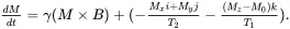
2.7 BLOCH EQUATION
When it can be assumed that the change of the magnetization following excitation is independently caused by external magnetic fields and relaxation processes, the equation of motion of Mcan be written by combining Eq. (2.14) and Eq. (2.15), in the laboratory frame, as
 (2.18)
This is the well-known Bloch equation [7]. The first term is due to precessional motion and the second term is due to relaxation. While a precise evaluation of the spin system requires a quantum mechanical treatment, the Bloch equation provides a classical, phenomenological description for liquids and liquid-like systems where the Hamiltonian is of a simple magnetic (vector) form, for example, protons of water molecules in non-viscous liquids and many biological tissues.
Now we are ready to solve the Bloch equation under various conditions. First rewrite the vector equation into the component form, as
 (2.19a)
 (2.19b)
 (2.19c)
The above equations have the usual setup for the magnetic fields as
 (2.20a)
 (2.20b)
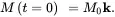
Thermal equilibrium ensures the initial condition of Min Eq. (2.19) as
 (2.21)
Note that as soon as Mis tipped away from its thermal equilibrium state, relaxation processes start. In most analyses, however, we consider only one event at a time – that is, when we use the B 1field to tip the magnetization, we do not consider the relaxation of the magnetization during the tipping process.
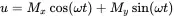
In order to better examine the solution of the Bloch equation (more precisely, to examine the spectral shapes of the waveform solutions), we will describe the magnetization in a rotating frame with an angular velocity ω about the z axis. In this x ′ y ′ z ′ frame, we have the component u in the direction of x′ and v in the direction of y ′. We can use the common rotation matrix in linear algebra to rewrite the transform matrix as
 (2.22a)
 (2.22b)
Note that Eq. (A1.23) is used in this clockwise rotation, which is consistent with the convention specified in Figure 1.3. (For a counterclockwise rotation, keep both terms of v positive and use a minus sign for the second term of u ; see Appendix A1.1).
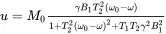
By writing the Bloch equation in this rotating frame and by setting the time derivatives in the equation equal to zero, we can solve the Bloch equation in the rotating frame. The solutions are
 (2.23a)
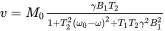 (2.23b)
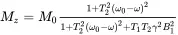 (2.23c)
2.8 FOURIER TRANSFORM AND SPECTRAL LINE SHAPES
Before we proceed to analyze the characteristics of the magnetization motion expressed in Eq. (2.23), let us pause for a moment to briefly mention two concepts that are essential to modern NMR, Fourier transform (FT) and spectral line shapes.
2.8.1 Fourier Transform
Fourier transform (defined mathematically in Appendix A1.2) utilizes the properties of sine and cosine functions and allows their periods to approach infinity. An operation by FT mathematically decomposes a generic function (often a function of time) into a complex-valued function of frequency, where each frequency can have a certain amplitude. When discussing the FT, one commonly uses the term domain to refer to the “space” where two functions are associated by FT, such as the time-domain function and its frequency domain counterpart. Figure 2.11 shows a sinusoidal oscillation in time and a delta function in frequency as a pair of Fourier functions. Both functions carry the same amount of information, where the frequency ( f 0) of the delta function is determined by the period ( T 0) of the oscillation, f 0= 1/ T 0. One can perform the FT for a multidimensional function (2D, 3D, …); one can also carry out an inverse FT that mathematically restores the original time-domain function from its frequency-domain representation. Table 2.2lists a few functions and their FT products.
Читать дальшеИнтервал:
Закладка:
Похожие книги на «Essential Concepts in MRI»
Представляем Вашему вниманию похожие книги на «Essential Concepts in MRI» списком для выбора. Мы отобрали схожую по названию и смыслу литературу в надежде предоставить читателям больше вариантов отыскать новые, интересные, ещё непрочитанные произведения.


Обсуждение, отзывы о книге «Essential Concepts in MRI» и просто собственные мнения читателей. Оставьте ваши комментарии, напишите, что Вы думаете о произведении, его смысле или главных героях. Укажите что конкретно понравилось, а что нет, и почему Вы так считаете.