Stephen J. Mildenhall - Pricing Insurance Risk

The algorithm’s computations can be visualized using a Lee diagram, as shown in Figure 3.13. The horizontal axis shows events and their cumulative probabilities (in 1/16ths and decimals). The width of each event corresponds to its objective probability, ΔS in the table. The vertical axis shows potential outcomes from 1 to 100. The horizontal black lines show the outcome X for each event. In this case, there are nine events with nine distinct outcomes. The shaded area shows the chances each unit of assets is needed to fund an event. For example, the 99th and 100th units are only at risk from (or needed to fund) event j = 9, which has outcome 100 (upper right-hand corner). We might say these units are potentially consumed by event j = 9. The eight units 91–98 are at risk from events j = 8 and j = 9. The step heights of the shaded area correspond to ΔX in the table and ΔX7 for row j = 7 is shown. At the bottom of the graph, the first unit of assets is needed to fund events j = 2 through 9. Event j = 1 has a zero loss, which does not require any assets. The plots in Figure 3.11 show the same function (different data values) rotated by 90 degrees to make the interpretation as ∫S(x)dx clearer.

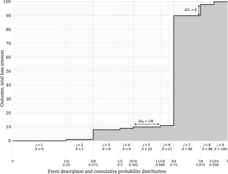
Figure 3.13 Lee diagram showing relationship between differen asset layers and the events they fund.

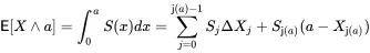
Given the increasing sequence X j, it is convenient to define j(a)=max{j:Xja . For example, j(90)=6 and j(91)=7. It is used in calculations as follows. To compute the limited expected value of X at a > 0, the survival function form evaluates

(3.12)

because ΔXj is the forward difference. It computes the integral as a sum of horizontal slices, e.g. the ΔX7 block in Figure 3.13. For a = 0 obviously E[X∧0]=0. For a=∞, j is set to j + 1, where j is the maximum index with S(Xj)>0, resulting in the unlimited E[X].

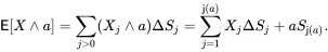
The outcome-probability form is

(3.13)

It computes the integral as a sum of vertical slices, e.g. the ΔS5 block in Figure 3.13.

When a = 80,

Table 3.4shows the above calculations through the simple expedient of replacing X values with X∧a and recomputing other columns that depend on X . Notice that columns involving S still use X ’s survival function. Numbers changed from Table 3.2are displayed in bold.

Table 3.4 Computing the limited expected value of X, limited to a = 80. X’ refers to X∧ a but values related to S are unchanged

j	X'	ΔX'	ΔS	S	X'ΔS	SΔX'
0	0	1	0.25	0.75	0	0.75
1	1	7	0.125	0.625	0.125	4.375
2	8	1	0.125	0.5	1	0.5
3	9	1	0.0625	0.4375	0.563	0.438
4	10	1	0.125	0.3125	1.25	0.313
5	11	69	0.0625	0.25	0.688	17.25
6	80	0	0.125	0.125	10	0
7	80	0	0.0625	0.0625	5	0
8	80	0	0.0625	0	5	0
Sum			1		23.625	23.625

An ice cream manufacturer wants to introduce a product that customers will prefer over existing ones. It would be very helpful to have a way of predicting customer ice cream preferences. As far as a customer is concerned their preference may be very simple and intuitive: “this brand tastes better!” That preference is not expressed in a way that the manufacturer can use to predict customer responses to a new product. However, through taste tests the manufacturer is able to determine general principles which do predict the preferences of most customers. For example, most customers prefer ice cream with a higher fat content and natural rather than artificial ingredients. This information is a good start but ideally the ice cream manufacturer can find a way to represent it numerically—an ice cream measure, if you will—which will enable them to analyze it much more easily.

Risk preferences have many parallels with ice cream preferences. Both are somewhat idiosyncratic and personalized—but some general principles about them can be determined, although it is harder for risk since there is no simple taste test to elicit risk preferences. Like ice cream manufacturers, risk management professionals would benefit from having a risk measure that quantifies a true risk preference and allows them to predict how individuals act. In this section, we try to find such risk measures. It is important to note that risk preferences are opposite to ice cream preferences in the sense that better ice cream is preferable, whereas more risk is not.

Formally, a risk measureis a real-valued functional on a set of random variables that quantifies a risk preference—the way an individual or group of individuals decides risk questions. The random variables represent risks, and the risk measure conducts a taste test; given two, it predicts which one is preferred, i.e. has lower risk. A risk capital formula, such as NAIC RBC or Solvency II SCR, and a classification rating plan are archetypal risk measures. Section 6.5 provides a compendium of other standard risk measures.

A risk preferencemodels the way we compare risks and how we decide between them. It captures our intuitive notions of riskiness and converts them into a form we can use to predict future preferences. Using the ice cream analogy, the manufacturer needs to convert “this tastes better” into a series of preferences about ice cream ingredients, which can be used to predict the desirability of a new product.

Risk preferences are defined on a set of loss random variables S. We write X⪰Y if the risk X is preferredto Y . If X⪰Y and Y⪰X we are neutral between X and Y .

A risk preference for insurance loss outcomes needs to have the following three properties.

1 Complete (COM) for any pair of prospects X and Y either X⪰Y or Y⪰X or both, that is, we can compare any two prospects.

2 Transitive (TR) if X⪰Y and Y⪰Z then X⪰Z.

3 Monotonic (MONO) if X≤Y in all outcomes then X⪰Y.

The second property ensures the risk preference is logically consistent. The third reflects the reality that large positive outcomes for losses are less desirable than small ones. If X⪰Y then X is generally smaller or tamer than Y . The third property also ensures the risk preference takes into account the volume or size of loss, even when there is no variability. For example a uniform random loss between 0 and ¤1 million is preferred to a certain loss of ¤1 million, even though the former is variable and the latter is fixed.

Читать дальше