Stephen J. Mildenhall - Pricing Insurance Risk

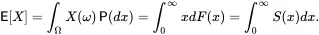
Figure 3.3 Different ways of computing expected losses for a sample discrete distribution. Each event is equally likely.

Consider a simple discrete space Ω={ω1,…,ω6} with six equally likely sample points. Let X be the loss random variable defined on Ω with outcomes 1,9,4,4,2, and 4.

The mean loss is 4, which can be seen by summing the losses, 24, and dividing by the number of outcomes or as the probability weighted sum of outcomes 1/6+2/6+4/2+9/6. Five ways of looking at X are illustrated in Figure 3.3.

Figure 3.3 panels (a) and (b) show the explicit representation. The outcomes are labelled by sample point. The two views illustrate that sample points do not have a natural ordering. We can compute the mean by summing over sample points, E[X]=∑ω∈ΩX(ω)Pr(ω). Event probabilities correspond to bar widths. We call this the event-outcome form.

Panel (c) is a Lee diagram. Compared to panel (b), it uses dual implicit labels for each outcome—its probability of nonexceedance Pr(X≤x)—in place of explicit events.

Panel (d) plots the survival (exceedance probability) function, S ( x ), against the outcome x . The width of the vertical bars equals the difference of the sorted outcome values. Using (d), we can compute the mean in the usual way as the sum-product of loss outcome and probability: ∑ixiPr(X=xi), since Pr(X=xi)=Pr(X>xi−1)−Pr(X>xi)=S(xi−1)−S(xi). Each area is exactly the same as in (c), just rotated by 90 degrees clockwise. We call this the outcome-probability form.

The orientation of the Lee and event-outcome diagrams stresses that the outcome loss is a function of the event rank or description. Lee’s orientation is more natural in many contexts than panels (d) or (e), and is used throughout the remainder of the book.

Panel (e) shows the same function as (d), but uses horizontal bars with heights equal to outcome probabilities, i.e. the differences of the survival function. Using (e), we can compute the mean as E[X]=∫0∞S(x)dx, by considering the chances each width-one outcome layer on the horizontal axis is used to pay a loss. The first layer is always used because all outcomes are ≥1. The second layer is used by five out of six outcomes, so 5/6 probability, the third and fourth by 4/6, etc. There is no possibility of a loss above 9. We call this the survival function form.

The total areas in panels (d) and (e) are the same but are divided up differently.

Converting the expressions for E[X] into integral form yields three equations for the mean:

(3.1)

The first integral corresponds to panels (a) and (b), the second to (d), and the last to (e). When X has a density f , ∫0∞xdF(x)=∫0∞xf(x)dx. Using xdF ( x ) is more general than xf(x)dx and allows for jumps in F , see Appendix A.4. We prefer to use xdF ( x ) unless the density exists and needs emphasizing.

The equivalence between the last two expressions in Eq. 3.1relies on integration by parts, ∫udv=uv−∫vdu, applied with u = x and v = S ,

since xS(x)→0 as x→∞ when X has a mean. Note that dS=−dF, accounting for the sign change.

Remark 16The expression ∫0∞S(x)dx for the mean is well known to life actuaries via the expression ex=∑tpt x for curtate future lifetime in terms of survival functions. The average future lifetime is the sum of the probability of surviving to each future age. Count the birthdays!

Exercise 17 Figure 3.3does not show the implicit representation. Plot it. What are the horizontal and vertical axes?

Exercise 18Let X be a Bernoulli random variable defined on Ω=[0,1] by X(ω)=0 for ω < 0.4 and X(ω)=1 for ω≥0.4. What are P(X=0), P(X=1), and E[X]? Plot X and its distribution and survival functions, and its Lee function. Clearly label all axes and the value of each function at any jump points. Repeat the exercise for Y defined by Y(ω)=0 if ω∈[0,0.1)∪[0.25,0.35)∪[0.5,0.6)∪[0.75,0.85) and Y(ω)=1 otherwise.

Solution. X and Y define different random variables but they have the same distribution and survival functions, and the same implicit and dual implicit representations. They are both Bernoulli(0.6) variables, with P(X=0)=0.4, P(X=1)=0.6, and mean E[X]=0.6. Figure 3.4 shows the requested plots. Strictly, the vertical segments are not part of the function graphs. The dot indicates the value of each function at jumps.

Figure 3.4 The random variables, distribution and survival functions, and Lee diagram for two identically distributed Bernoulli random variables.

Exercise 19A model produces 100 equally likely events that it labels by an event identifier. The events define a sample space Ω={0,…,99} and probability Pr({ω})=1/100. The model defines two identically distributed, dependent random variable outcomes

with sum

1 Create the model in a spreadsheet and confirm E[X]=28 and E[Xi]=14.

2 Plot X1, X2, and X as functions of ω=0,1,…,99.

3 Plot the survival functions, as functions of the outcome x.

4 Plot the Lee diagrams, as functions of probability p.

5 Are the random variables different? The survival functions? The Lee diagrams?

We return to this example in Chapter 15.

Solutions.Figures 3.5–3.7 show the random variables, the survival functions, and the Lee diagrams. The random variables are all distinct, but the survival function and Lee diagrams for each line are the same.

Figure 3.5 Random variables, functions of an explicit state.

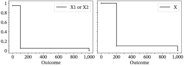
Figure 3.6Survival functions of the outcome.

Figure 3.7 Lee diagrams, function of a dual implicit state.