Philip Hofmann - Solid State Physics

(1.20)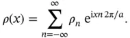

To ensure that is still a real function, we require that

(1.21)

that is, that the coefficient must be the complex conjugate of the coefficient . This description is more elegant than the one with the sine and cosine functions. How is it related to the reciprocal lattice? In one dimension, the reciprocal lattice of a chain of points with lattice constant is also a chain of points, now with spacing [see Eq. (1.17)]. This means that we can write a general reciprocal lattice “vector” as

(1.22)

where is an integer. Exactly these reciprocal lattice “vectors” appear in Eq. (1.20). In fact, Eq. (1.20)is a sum of functions with a periodicity corresponding to the lattice vector, weighted by the coefficients . Figure 1.11illustrates these ideas by showing the lattice and reciprocal lattice for such a chain as well as two lattice‐periodic functions, both in real space and as Fourier coefficients on the reciprocal lattice points. The advantage of describing these functions by the coefficients is immediately obvious: Instead of giving for every point in a range of , the Fourier description consists of just three numbers for the upper function and five numbers for the lower function. Actually, these even reduce to two and three numbers, respectively, because of Eq. (1.21).

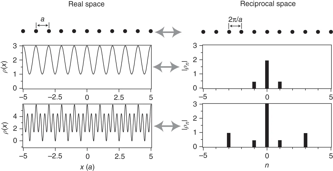
Figure 1.11 Top: A chain with a lattice constant as well as its reciprocal lattice, a chain with a spacing of . Middle and bottom: Two lattice‐periodic functions in real space as well as their Fourier coefficients. The magnitude of the Fourier coefficients is plotted on the reciprocal lattice vectors they belong to.

The same ideas also work in three dimensions. In fact, one can use a Fourier sum for lattice‐periodic properties that corresponds to Eq. (1.20). For the lattice‐periodic electron concentration 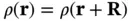, we get

(1.23)

where are the reciprocal lattice vectors.

Thus we have seen that the reciprocal lattice is very useful for describing lattice‐periodic functions. But this is not the whole story: The reciprocal lattice can also simplify the treatment of waves in crystals in a very general sense. Such waves can be X‐rays, elastic lattice distortions, or even electronic wave functions. We will come back to this point at a later stage.

Turning back to the specific problem of X‐ray diffraction, we can now exploit the fact that the electron concentration is lattice‐periodic by inserting Eq. (1.23)in our expression from Eq. (1.11)for the diffracted intensity. This yields

(1.24)

Let us inspect the integrand. The exponential represents a plane wave with a wave vector . If the crystal is very big, the integration will average over the crests and troughs of this wave and the result of the integration will be very small (or zero for an infinitely large crystal). The only exception to this is the case where

(1.25)

that is, when the difference between incoming and scattered wave vector equals a reciprocal lattice vector. In this case, the exponential in the integral is 1, and the value of the integral is equal to the volume of the crystal. Equation 1.25is often called the Laue condition. It is central to the description of X‐ray diffraction from crystals in that it describes the condition for the observation of constructive interference.

Looking back at Eq. (1.24), the observation of constructive interference for a chosen scattering geometry (or scattering vector ) clearly corresponds to a particular reciprocal lattice vector . The intensity measured at the detector is proportional to the square of the Fourier coefficient of the electron concentration . We could therefore think of measuring the intensity of the diffraction spots appearing for all possible reciprocal lattice vectors, obtaining the Fourier coefficients of the electron concentration and reconstructing this concentration from the coefficients. This would give us all the information needed and thus conclude the process of structure determination. Unfortunately, this straightforward approach does not work because the Fourier coefficients are complex numbers. Taking the square root of the intensity at the diffraction spot therefore gives the magnitude, but not the phase of . The phase is lost in the measurement; this is known as the phase problemin X‐ray diffraction. To solve an unknown structure, one has to find a way to work around it. One simple approach for this is to calculate the electron concentration for a structural model, obtain the magnitude of the values and thus also the expected diffracted intensity, and compare this to the experimental result. Based on the outcome, the model can be refined until the agreement is satisfactory.