Julian Barbour - The End of Time - The Next Revolution in Physics

In Chapter 3 we imagined tipping triangles out of a bag. That exercise was presented because it mimics one of the ways in which we can interpret a quantum state. Imagine now that the blue mist has the distribution shown in Figure 40. To avoid problems with infinite numbers of configurations, we divide up Q by a grid of cells sufficiently fine that ψ hardly changes within any one of them (Figure 40, on the right). The intensity of the blue mist at the central point of each cell then gives the relative probability of the nearly identical configurations in that cell. On a piece of cardboard, let us depict one of these configurations (as shown on the left in Figures 39 and 40). This will serve as the representative of all the configurations of that cell. For the grid in the figure with 100 cells, there are 100 relative probabilities whose sum should be conveniently large, say a million. Then we shall not distort things seriously by replacing exact relative probabilities like 127.8543... by the rounded-up integer 128.

We now imagine putting into a bag the number of copies of each representative configuration equal to its rounded probability, 128 for example. In quantum mechanics, performing a measurement to determine the positions of both particles is like drawing at random one piece of cardboard from the bag. We get some definite configuration. In the process, we destroy the wave function and replace it by one entirely concentrated around the configuration we have found. If we recreate the original wave function, by repeating the operations that we used to set it up, and repeat the experiment millions of times, then the relative frequencies with which the various configurations are ‘drawn from the bag’ will match, statistically, the calculated relative probabilities.

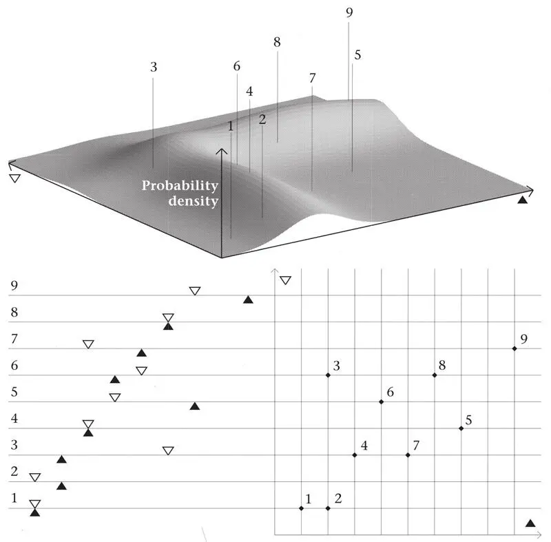
Figure 40.Like Figure 39, this shows nine different configurations of two particles (black and white triangles) on a line and the points corresponding to them in the configuration space Q (on which a grid has been drawn). A possible distribution of the intensity of the blue probability mist is shown as the height of a surface over Q in the top part of the figure (you are seeing the surface in perspective from above, and rotated). In the state of the system shown here, the probabilities for configurations 4, 6 and 9 are high, while 5 has a very low probability.

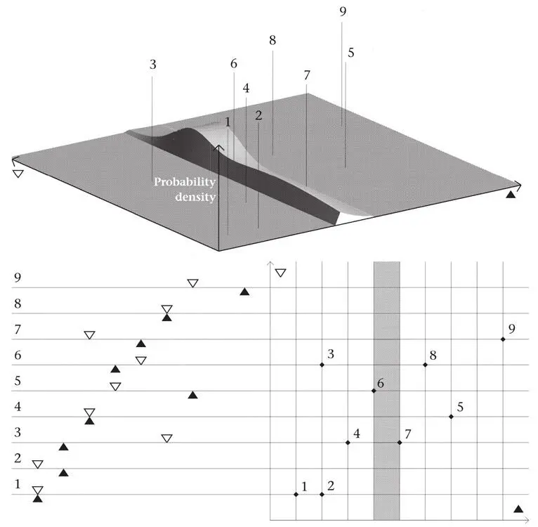
Figure 41 (a).The effect of measuring, for the probability density of Figure 40, the position of the particle represented by the horizontal axis, and finding that it lies in the interval on which the vertical strip stands. All the wave function outside the strip is instantaneously collapsed.

This is only the start. We can select from a menu of different kinds of measurement. For example, we can opt to find the position of only one particle, which has remarkable implications for what we can say about the other one. Suppose first that we measure the position of just one of the particles. According to the quantum rules, this instantaneously collapses the wave function from its original two-dimensional ‘cloud’ to a one-dimensional profile (Figure 41). The point is that we now know the position of one particle to within some small error, so none of the wave function outside the narrow strip is relevant any longer. It is annihilated. If the particle whose position is measured is represented along the horizontal axis, only a vertical strip of ψ survives (Figure 41(a)); if the position of the other particle is measured, only a horizontal strip survives (Figure 41(b)).

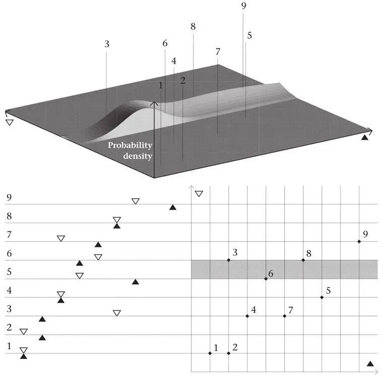
Figure 41 (b).The same for a position measurement of the other particle.

Either profile then gives conditional information. If we know where one particle is, the possible positions of the other are restricted to a narrow strip. The relative probabilities for the position of the second particle are determined by the values of ψ within the strip. Provided we know the original wave function, acquired knowledge about one particle sharpens our knowledge – instantaneously – about the other. This is the place to explain entangled states , or quantum inseparability (Box 12).

BOX 12 Entangled States

Figure 42 again shows our two-particle Q and two different quantum states. In the unentangled state at the bottom, all the horizontal ψ profiles are identical, and so are all the vertical profiles (only their shapes count). Such a wave function is said to be unentangled because if we gain information about particle 1 (black triangles) – that it is at some definite position – we do not gain any new information about particle 2 (white triangles). This is because all the horizontal profiles and all the vertical profiles are identical: they give identical relative probabilities. This is shown by two profiles that result from an exact position measurement of particle 1. Measurement on particle 1 leads to no new information about particle 2.

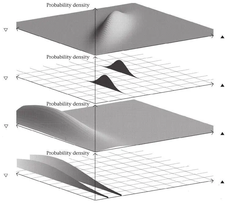
Figure 42.Entangled (top) and unentangled (bottom) states for two particles (black and white triangles).

Much more interesting is the entangled state at the top, for which the horizontal and vertical profiles are not identical. Figure 42 shows two profiles that result from exact position measurement of particle 1. They give very different probability distributions for particle 2: the gain in information about particle 2 is considerable. This is typical of quantum mechanics, since virtually all wave functions are entangled to a greater or lesser extent.

A particular feature of entangled states should be noted. Particles normally interact (affect each other) when they are close to each other. For the two-particle Q in Figure 39, the particles coincide on the diagonal line, and the region in which the particles are close to each other and can interact strongly is therefore a narrow strip around that line. However, the wave function of an entangled state may be located completely outside this region – the particles may be very far apart when one of them is observed. Yet the other particle is apparently immediately affected. It can jump to one or other of two hugely different possibilities. Moreover, if the ‘ridge’ in the top part of Figure 42 is made thinner and thinner, shrinking to a line, then position determination of one particle immediately determines the position of the other to perfect accuracy. Such situations are not easy to engineer for position measurements (and in general will not persist because of wave-packet spreading), but there are analogous situations for momentum and angular-momentum measurements that are easy to set up.

The facts discussed in Box 12 are immensely puzzling if we wish to find a physical and causal mechanism to explain how measurement on one particle can have an immediate effect on a distant particle. As I have already explained, innumerable interference phenomena indicate that, in some sense, the particles are, before any measurement is made, simultaneously present wherever ψ extends. Since there is no restriction on the distance between the particles, any causal effect on the second particle after the first has been observed would have to be transmitted instantaneously. However, relativity theory is supposed to rule out all causal effects that travel faster than the speed of light. Moreover, in the mid-1980s Alain Aspect in Paris performed some very famous experiments in which such wave-function collapses were tested, and the predictions of quantum mechanics confirmed with great accuracy. The experiments were so arranged that any physical effect would have had to be transmitted faster than the speed of light to bring about the collapse.