Jean-François Sigrist - Numerical Simulation, An Art of Prediction, Volume 2

“Nature has so much real wealth to unveil and humans have such a definitively superior potential for intelligence, that the combination of the two frankly gives hope […] Working with nature and not against it, we realize that the solutions are there, before our eyes and that they often prove to be simpler and less costly in energy […] We have divided by thirty our energy efficiency to produce food since the time of our grandparents… that sounds like a terrible insult to human intelligence” [ROS 18].

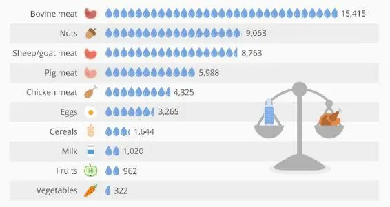
Figure 1.6. How thirsty is our food?

(source: https://www.statista.com/chart/9483/how-thirsty-is-our-food/ )

COMMENT ON FIGURE 1.6.– We use water in any productive activity, the amount consumed depending on two main factors: the climate of the production region and the agricultural practices developed there. For example, 35 L of water is needed to produce a cup of tea, 140 L for a cup of coffee, 75 L for a glass of beer and 120 L for a glass of wine; 2,400 L are consumed for the production of a hamburger, 40 L for a slice of bread and 13 L for a tomato (source: www.fao.org ) .

In the 21st Century, will numerical modeling contribute to the development of agricultural techniques that ensure a sufficient level of agricultural production for all humanity and limit the degradation of its environment?

In the richest countries, agriculture is becoming digital and modeling is a key focus of this change [WAL 18]. David Makowski, an expert in this field at INRA* , explains the objective:

“Germany, Australia, France, Italy, the United States and the Netherlands are the pioneering countries in the use of numerical modeling in agriculture, recently joined by China. Numerical simulation makes it possible to assess the impact of agricultural practices, soil quality and climate on yields and the environment. The applications are varied and allow farmers, companies and public agencies to estimate the performance of different production methods in different situations. Despite the sometimes significant uncertainty of their simulations, models are frequently used to predict the environmental impact of agriculture by assessing the emissions of particulate matter, greenhouse gases or pollutants due to agricultural practices”.

Numerical simulations in agronomy have used “mechanistic models” for two to three decades. These allow the functioning of crops to be described by means of equations; these, for instance, represent the production of biomass as a function of solar radiation, or the growth of plants as a function of soil temperature or humidity. Simulations make it possible to account for the physiological and biological dynamics of plants, on the scale of a plot or a set of cultivated lands. They can represent different agricultural practices and help to assess their impact on yields.

An example of modeling applicable to biological phenomena? The interaction model between hosts and biological control auxiliaries. It describes how biological populations, such as predators and their prey (aphids and ladybirds for example), evolve in an ecosystem. For example, it explains the development cycles of many species (animal, plant, etc.) in many environments, such as the marine phytoplankton (Figure 1.7).

The model consists of two differential equations, proposed independently by two mathematicians, the Austrian Alfred-James Lotka (1880–1949) and the Italian Vito Volterra (1860–1940), in 1925–1926. These equations are written as:

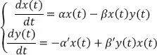
The equations describe the evolution of the prey and predator population, represented by variables x ( t ) and y ( t ). The first equation states that prey, having access to an unlimited source of food, would grow exponentially (this is rendered by the first term in the right-hand side of the equation αx ( t )), and are sometime faced with predators at certain occurrence (this is rendered by the second term of in the right hand side of the equation –βx ( t ) y ( t )). The second equation states that predators perish from natural death (this is rendered by the first term in the right-hand side of the equation –α′x ( t )), but grow by hunting prey (this is rendered by the second term of in the right-hand side of the equation +β′y ( t ) x ( t )).

Figure 1.7. Satellite image showing algae growth in a North Atlantic region (source: www.nasa.gov ). For a color version of this figure, see www.iste.co.uk/sigrist/simulation2.zip

COMMENT ON FIGURE 1.7.– In the waters of the North Atlantic, a large amount of phytoplankton, microscopic algae that play a role in the food chain of the marine ecosystem and contribute to the ocean carbon cycle, develops each spring and fall. The image is a photograph taken by NASA’s “Suomi” satellite on September 23, 2015. Blue spirals represent high concentrations of algae, waters loaded with microscopic creatures that contribute to the production of part of the planet’s oxygen .

The Lotka–Volterra equations have as unknown the populations of the competing species, the coefficients describe their survival and mortality rates. They predict a cyclical evolution of populations that is consistent with the observations (Figure 1.8). Many other equation-based models are available for studies of organic and agricultural systems. In recent years, data-based simulations have been developed to complement these models – nowadays, they use methods such as automatic learning techniques, discussed in Chapter 4of the first volume. Statistical models are based on an adjustment of equations to data and allow an empirical relationship between different quantities to be established.

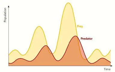
Figure 1.8. Typical evolution of the prey/predator populations as predicted by the Lotka-Volterra equations

Satellites, drones (Figure 1.9), sensors, field surveys: statistical models are based on a large number of data and it is the variety and diversity of the latter that gives credibility to predictions. Data used in statistical models are diverse: they describe the crop environment (e.g. topography and meteorology), farmers’ practices (e.g. frequency of watering or spreading), animal species behavior or plant species growth.

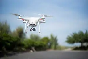
Figure 1.9. Agricultural drones are used to monitor crops and collect useful data to develop or validate certain simulations

(source: © Christophe Maitre/INRA/ www.mediatheque.inra.fr/ )

The models of each family complement each other, each providing information whose multimodel analysis makes it possible to identify trends [MAK 15]: