Michael Begon - Ecology

Source : After DeLong et al . (2010).

As another example, the allometric exponent in plants appears to be consistently different between, on the one hand, seedlings and the smallest plants, and on the other, larger saplings and adult plants – close to 1 for plants with masses less than 1 g and converging to 0.75 as masses exceed around 100 g ( Figure 3.34), though the particular mass values should not be taken too literally. In this case, the authors hypothesise that for larger plants, the photosynthetic machinery is distributed across surfaces (principally of leaves), whereas for smaller plants most or all of the tissue (and hence a volume) is photosynthetically active (Mori et al ., 2010). A curvilinear relationship has also been proposed for mammals, but this time with the opposite curvature, starting at 0.57 and rising to 0.87 (Kolokotrones et al., 2010).

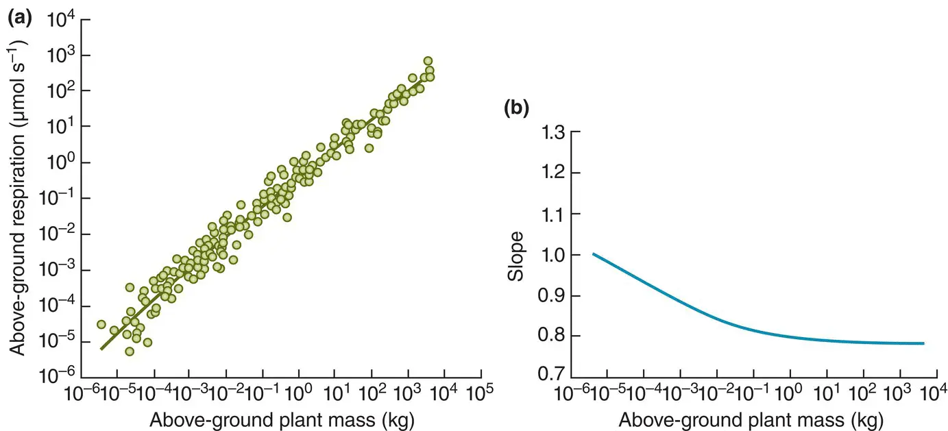
Figure 3.34 The allometric exponent of metabolism in plants decreases with plant size. (a) The relationship between temperature‐adjusted respiration rate and above‐ground plant mass across a wide range of masses on logarithmic scales. A curvilinear power function was fitted to the data, the changing slope of which is shown in (b).

Source : After Mori et al . (2010).

Note, to add a further perspective, that alongside SA and RTN theories, there is an equally long tradition of emphasising body composition as a driver of metabolic rate, with some organisms having a much higher proportion of structural, low‐metabolising tissue than others (see Glazier, 2014); and other studies again have emphasised the importance of changing shape (which the simpler theories assume remains constant) and show that the shifting patterns of metabolic rates with shape support the SA but not the RTN theories of metabolic scaling (Hirst et al ., 2016). However, particular values of b , and the truth or otherwise of the hypotheses proposed to explain them, are less important than the more general point that an organism’s rate of metabolism reflects a whole host of constraints and demands, and different factors will therefore dominate in their effects in different organisms, and at different times, and b will therefore vary. It is unwise to seek a single, universal value for b , or a single, simple basis for all metabolic scaling. The key message, picked up again in later chapters, is that the scaling of metabolic rate plays a key role in the dynamics at all levels of ecological organisation, from the individual to the whole community.

Much of ecology is concerned with numbers and changes in numbers. Which species are common and which species rare? Why? Which species remain constant in abundance and which vary? Why? How can we reduce the numbers of a pest? Or prevent reductions in the numbers of a rare but valued species? At the heart of all such questions, there is a fundamental ecological fact of life:

(4.1)

That is, the numbers of a particular species presently occupying a site of interest ( N now) is equal to the numbers previously there ( N then), plus the number of births between then and now ( B ), minus the number of deaths ( D ), plus the number of immigrants ( I ), minus the number of emigrants ( E ).

This defines the main aim of ecology: to describe, explain and understand the distribution and abundance of organisms. Ecologists are interested in the number of individuals, the distributions of individuals, the demographic processes (birth, death and migration – also often referred to as vital rates ) that influence these, and the ways in which these demographic processes are themselves influenced by environmental factors.

individuals differ

Among the simplifications in our ecological fact of life is the implicit assumption that all individuals are alike (since all we need do is count them), which is patently false on a number of counts. First, almost all species pass through a number of stages in their life cycle: eggs, larvae, pupae and adults in many insects; seeds, seedlings and photosynthesising adults in plants; and so on. The different stages are likely to be influenced by different factors and to have different rates of migration, death and, of course, reproduction. Second, even within a stage, individuals can differ in ‘quality’ or ‘condition’. The most obvious aspect of this is size, but it is also common, for example, for individuals to differ in the amount of stored reserves they possess.

unitary and modular organisms

Uniformity amongst individuals is especially unlikely when organisms are modular rather than unitary . In unitary organisms – mammals, birds, insects and so on – form and the succession of phases in the life cycle are predictable and ‘determinate’. That is, all dogs have four legs and each squid has two eyes, and dogs and squid that lived longer would not develop more of them. Similarly, we humans pass through an embryonic stage of nine months, a growth phase of around 18 years incorporating a prereproductive phase of 12 or so years, a reproductive phase lasting perhaps 30 years in females and rather longer in males, followed finally by a phase of senescence. Death can intervene at any time, but for surviving individuals the succession of phases, and even mostly the timing of phases, is, like form, entirely predictable.

But none of this is so simple for modular organisms such as trees, shrubs and herbs, chain‐forming bacteria and algae, corals, sponges, and very many other marine invertebrates ( Figure 4.1). These grow by the repeated production of ‘ modules’ (leaves, coral polyps, etc.) and almost always form a branching structure. Most, following a juvenile phase, are rooted or fixed, not motile, and both their structure and their precise programme of development are not predictable but ‘indeterminate’. After several years’ growth, depending on circumstances, the same germinating tree seed could either give rise to a stunted sapling with a handful of leaves or a thriving young tree with many branches and thousands of leaves. It is modularity and the differing birth and death rates of modules that give rise to this plasticity. Reviews of the growth, form, ecology and evolution of a wide range of modular organisms may be found in Harper et al . (1986), Hughes (1989) and Collado‐Vides (2001).

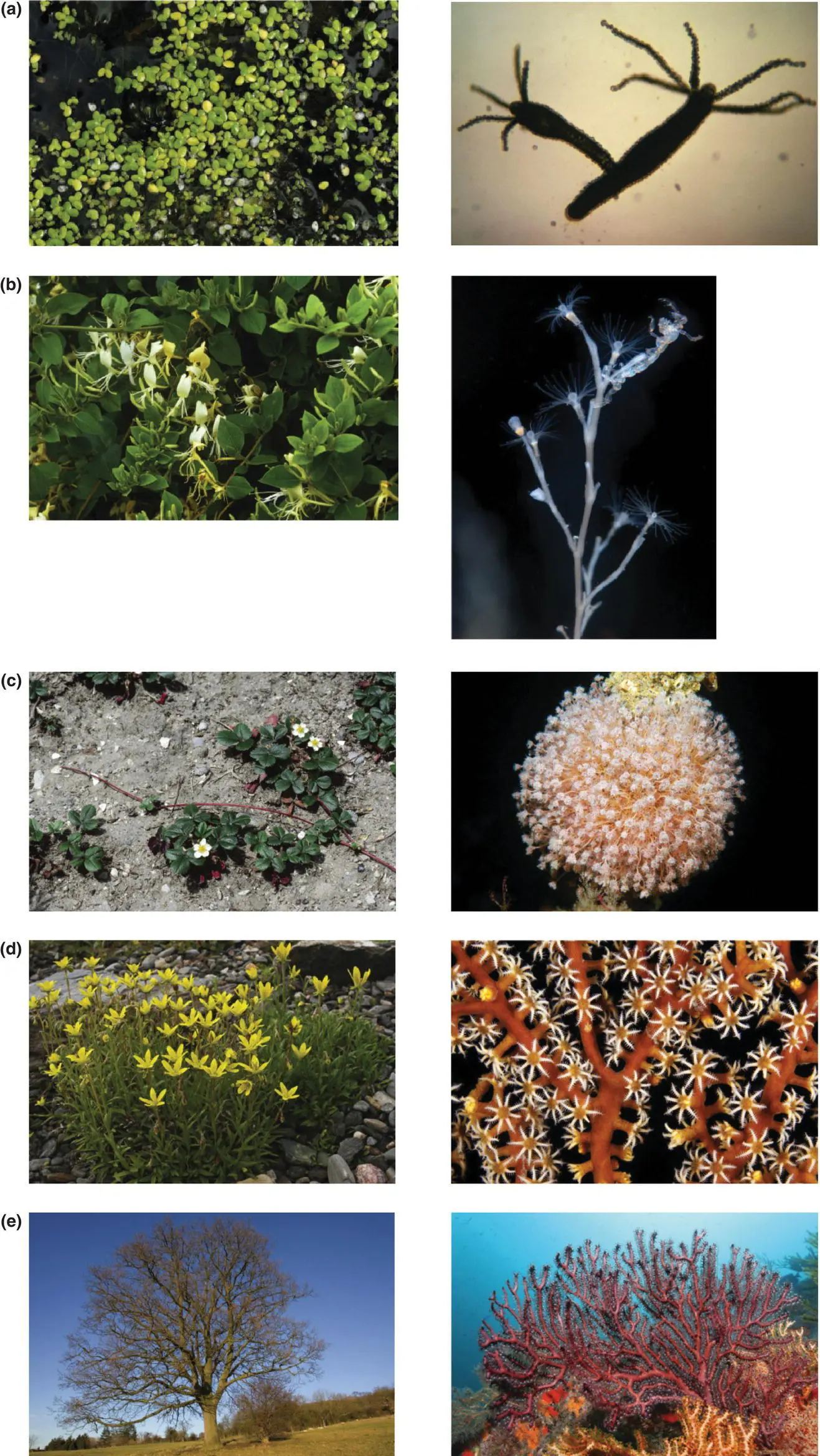
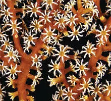
Figure 4.1 Modular plants (left) and animals (right) show the underlying parallels in the various ways they may be constructed.(a) Modular organisms that fall to pieces as they grow: duckweed ( Lemna sp.) and Hydra sp. (b) Freely branching organisms in which the modules are displayed as individuals on ‘stalks’: a vegetative shoot of a higher plant ( Lonicera japonica ) with leaves (feeding modules) and a flowering shoot, and a hydrozoa ( Extopleura larynx ) bearing both feeding and reproductive modules. (c) Stoloniferous organisms in which colonies spread laterally and remain joined by ‘stolons’ or rhizomes: strawberry plants ( Fragaria ) reproducing by means of runners, and a colony of the hydroid Tubularia crocea . (d) Tightly packed colonies of modules: a tussock of yellow marsh saxifrage ( Saxifraga hirculus ), and a segment of the sea fan Acanthogorgia . (e) Modules accumulated on a long persistent, largely dead support: an oak tree ( Quercus robur ) in which the support is mainly the dead woody tissues derived from previous modules, and a gorgonian coral in which the support is mainly heavily calcified tissues from earlier modules.