Position, Navigation, and Timing Technologies in the 21st Century

In the present setting of dead reckoning from a known location, the initial stationary TOA measurements can be accumulated into a “deterministic” reference. The time difference with respect to such a reference at a fixed time point as in Eq. (40.8) is akin to applying a well‐calibrated bias to all subsequent measurements, which can then be treated as approximately “uncorrelated.” This initial measurement error, if not calibrated out to an insignificant level, would make subsequent time‐difference measurements time‐correlated. Because it is constant, albeit random, it can be viewed as an unknown bias and modeled as an extra state to the positioning Kalman filter.

Strictly speaking, no matter how well a parameter is calibrated, the subsequent measurements can be time‐correlated via the residual calibration errors. Furthermore, time differencing can also be applied continuously to consecutive measurements, that is, between t +1 and t , rather than between t and t 0= 0 as in Eq. (40.8). Consecutive time differences between times ( t +1 and t ) and ( t and t −1) are correlated through the common epoch t . The standard Kalman filter cannot be applied to consecutive time‐difference measurements because the measurements are correlated. In [92], a fixed‐lag smoother was used where the previous position is introduced as an extra state. With both the current and previous positions in the filter, the position difference becomes directly observable by the time differences of carrier phase measured at the current and previous epochs [92]. A similar formulation can be used for SOOP when processing consecutive time differences of phase and/or range measurements.

In the field test environment depicted in Figure 40.17, a radio receiver with seven synchronous channels is installed in a minivan together with a battery‐powered data recording system. One channel is assigned to GPS L1, which serves as the reference; one channel to a CDMA cell tower in the PCS band; and the other five channels to five DTV stations. One DTV station (605 MHz) is on Monument Peak in the south, four DTV stations (563, 617, 623, and 647 MHz) are on Sutro Tower in the north, and one CDMA cell tower (1933.75 MHz) is also in the north. Since we were driving from the south to north, the range to the DTV station on Monument Peak was increasing while the ranges to the other six sources in the north were decreasing.

Figure 40.23(a) shows the relative ranges to the DTV and CDMA sources. The vehicle was stationary for the first 40 s and then moving about 300 m in 50 s (at a speed of 15 mph on average). As shown in Figure 40.23(b), the initial transients settled after 0.5 s for the DTV channels and after 3 s for the CDMA channel. Except for the DTV channel at 617 MHz, which exhibits large variations (−5 to 10 m), the others are small (±2 m). In fact, the standard deviations during the stationary period are 0.78, 0.88, 1.67, 4.13, 1.15, and 1.49 m, respectively.

Figure 40.23(c) shows the relative ranges during motion. Due to fast fading, the range measurements are noisier in motion than during stationary (about four times larger). As discussed above, the range to the DTV channel at 605 MHz on Monument Peak (in the south) is opposite to the other ranges (in the north), with a maximum peak‐to‐peak variation of 70 m but mostly of 20 m. The DTV channel at 647 MHz shows a sharp change of 120 m after moving and toward the end. The other three DTV channels on Sutro Tower show similar behaviors. The largest separation in range is about 50 m, which is consistent with their distances calculated from their coordinates. It is remarkable to note that the CDMA range also fits nicely with the DTV ranges.

In the following processing, we excluded the DTV channel at 647 MHz due to large deviations. Figure 40.23(d) shows the least squares (LS) solution (green) based on the raw relative range measurements shown in Figure 40.23(a), the Kalman filter (KF) estimate (red), and the GPS solution (blue). As explained in Section 40.4.1, large errors are expected in the cross‐range direction due to the poor geometry.

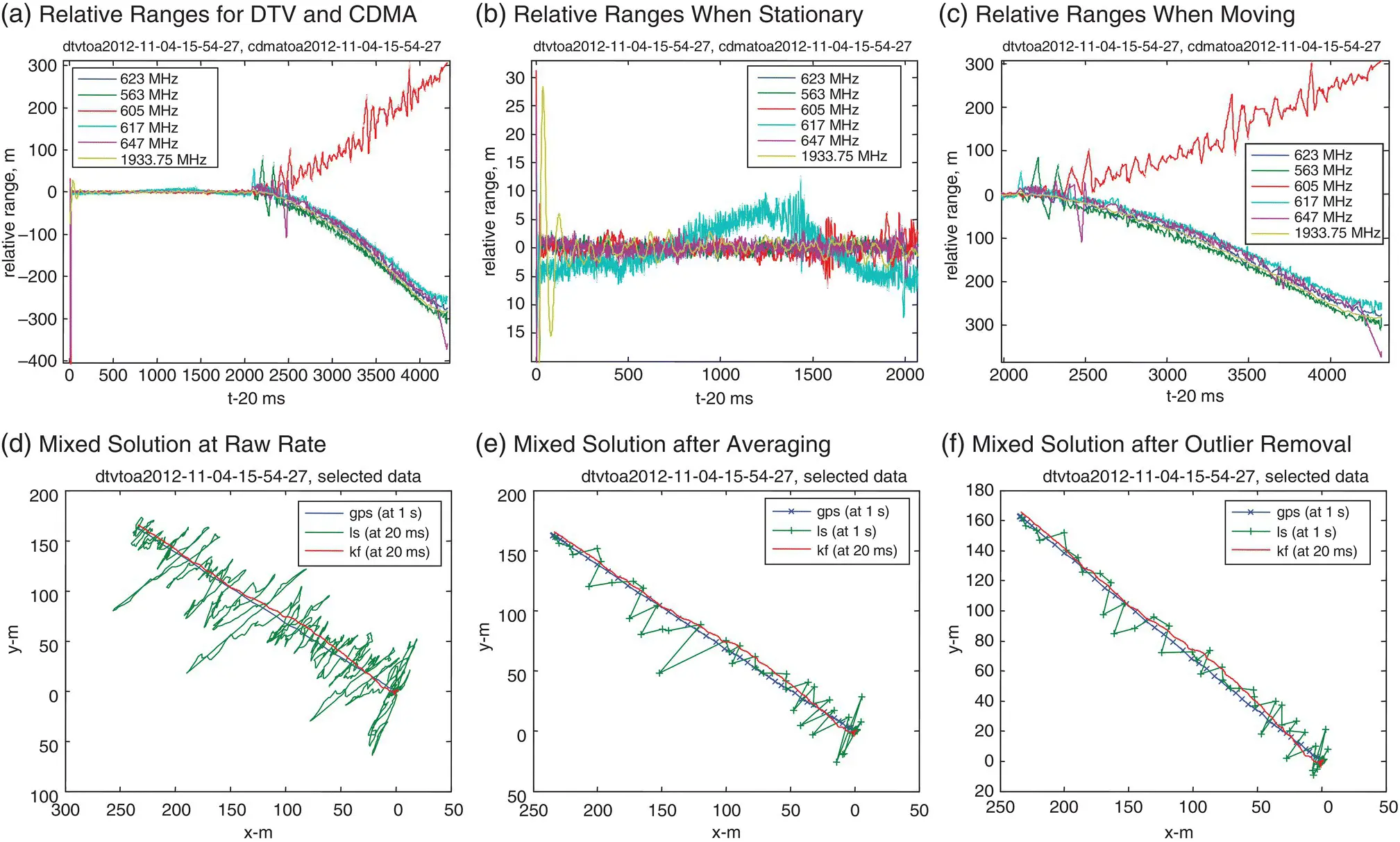
Figure 40.23 Radio dead-reckoning (relative positioning) with mixed signals of opportunity (SOOP).

Figure 40.23(e) shows the LS solution (green) after averaging with an equivalent interval of 1 s to be compatible with the GPS solution at 1 Hz. Large deviations in the middle of trajectory are likely caused by the range measurements of the DTV channel at 605 MHz. After a threshold testing (±15 m) applied to the relative range predictions to remove measurement outliers, the large deviations appearing in Figure 40.23(e) are eliminated, and the resulting trajectory is shown in Figure 40.23(f). Averaged along the trajectory, the mean error of the SOOP‐alone solution versus the GPS‐alone solution is 1.68 m with a standard deviation of 3.78 m and a maximum error of about 12 m.

Radio propagation in urban environments is known to be subject to two types of fading [42, 83]: large‐scale fading, which is range dependent (this range dependency is the main idea behind the RSS‐based positioning mentioned earlier), and small‐scale fading, which occurs over short distance (several wavelengths) and a short period of time (seconds). In small‐scale fading, the received signal is subject to rapid changes, mainly caused by multipath signals with constructive and destructive additions. It causes signal dispersions in time, frequency, and angle of arrival, which are known as delay spread, Doppler spread, and angular spread, respectively. It is this small‐scale fading that severely hampers mobile tracking of SOOP such as cellular and DTV signals. An agile radio receiver is therefore desired to implement fast acquisition and reacquisition schemes to coast through the “holes” of deep fading with instantaneous recovery after a complete signal loss, a correlator structure commensurate with the variable delay experienced by the receiver, and tracking loop parameters optimized to balance out dynamic tracking versus noise performance requirements.

In urban environments, the direct signal may be blocked or severely attenuated while strong multipath components are omnipresent. The conventional strategy of picking up the peak among a limited number of early and late correlation values, though still valid for communications purposes to demodulate the data bits, is error prone for LOS timing, which may create bias in range measurements and, even worse, outliers. Holistic processing of the entire CIR, as described in Section 40.2.2[51, 52], is more promising for dealing with multipath and NLOS signals [27, 94, 95]. Outliers can be treated with robust estimation methods [96–98].

Mixed SOOP are capable of offering a stand‐alone solution in a rather poor geometry, as demonstrated in the examples presented. It can be further integrated with other sensors and used to assist GNSS for more robust operations. The GNSS and SOOP aiding is mutual. All missions start from a known initial condition just like an inertial navigation system that is initialized with the position, velocity, and attitude at the starting point. When GNSS is available, its solution can help SOOP determine the hearable transmitter location (akin to mapping and intelligence gathering) and calibrate the time offset and drift rate. As part of an integrated navigation system, the GNSS‐based solution can relax the stringent requirement otherwise placed on the number of independent SOOP and their geometric distribution. The continuity and availability of a hybrid solution can be ensured based on one to two GNSS signals, one to two DTV signals, and/or one to two cellular signals with a reasonably good geometry and signal quality.