Position, Navigation, and Timing Technologies in the 21st Century

Source: Reproduced with permission of Stanford University.

Two TV antennas (separated by 1 m) are mounted on the roof of a car, which is driven at a speed between 0 to 50 km/h for 5 min including three stationary segments from 0–10 s, 70–110 s, and 285–300 s as shown in Figure 40.21(a). The evolution of the absolute value of the correlation function over time is shown in Figure 40.21(b), where the horizontal axis is the time, the vertical axis is the delay, and the correlation strength is color‐coded, with the dark red representing the strongest return (0 dB) and the dark blue representing the weakest return (−30 dB). Clearly, the correlation peak is spread out, an indication of the presence of multipath signals, some of which have rather long delays. There is a short horizontal segment with weak return (due to stopping from 70 to 110 s) where the direct signal may be blocked or attenuated to a level comparable to multipath.

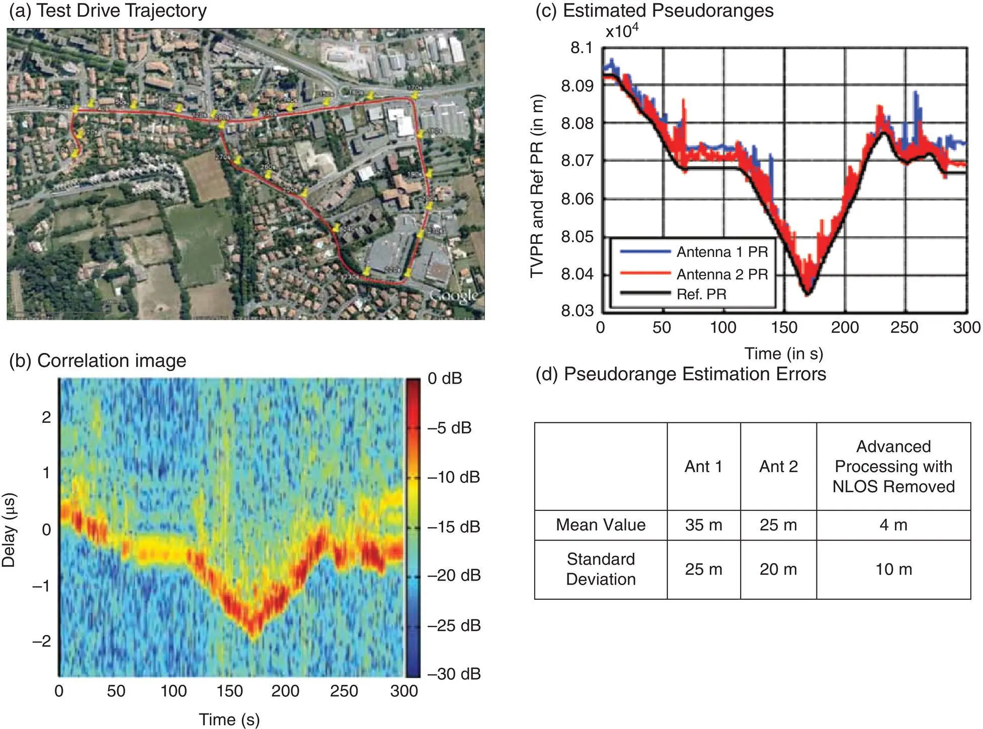
Figure 40.21 Results of field tests for ranging with DVB‐T signals [8].

Source: Reproduced with permission of Inside GNSS Media LLC.

Figure 40.21(c) shows the pseudoranges estimated from DVB‐T signals received by the two antennas (blue from the first antenna and red from the second) compared to the reference pseudorange (back) computed from the GPS‐based car position (real‐time kinematic or RTK) and the known transmitter location. The pseudorange errors are mostly positive (i.e. pseudorange in excess of the true value), a clear indication of NLOS errors. The blue curve from the first antenna shows larger bias and spikes than the second, particularly during the static periods (around 100 s and at the end). The errors are very different (up to 150 m) even though they are so close (separated only by 1 m), again a clear sign of location‐dependent multipath errors.

In Figure 40.21(d), the table lists the mean and standard deviation of 35 m and 25 m for the first antenna and 30 m and 20 m for the second, respectively. Advanced measurements processing, which can remove the NLOS signals [9], significantly improves the accuracy, leading to a mean and standard deviation of 4 m and 10 m, respectively.

Using ATSC‐8VSB signals as an example, this section first analyzes the effect of transmitter‐receiver geometry on positioning accuracy in Section 40.4.1to highlight the needs for mixed SOOP. Mobile test results for radio dead reckoning with mixed SOOP are presented in Section 40.4.2. A number of practical issues are discussed in Section 40.4.3as part of future research.

Range‐based positioning accuracy is determined by ranging errors on the one hand and by the ranging geometry on the other hand. For the 2D case, the circular probably error (CEP) is given by

(40.7)

where σ is the standard deviation of the ranging errors, and GDOP is the geometric dilution of precision.

The ranging error σ is determined by the SNR, signal bandwidth, signal structure, and multipath, among others, which can be reduced by good antenna and RF front‐end designs with low noise figure (NF) and advanced baseband signal processing algorithms. For ATSC‐8VSB signals, ranging is based on the PN codes in the field sync segment. As shown in Figure 40.2, the chipping rate is 10. 76 Mcps, and the code repeats once every 24.2 ms. If the ranging accuracy is at 10% of a code chip, the expected accuracy is about 3 m; and field tests show a standard deviation from 3 to 12 m, depending on the test environments and receiver mobility. For DVB‐T signals, the refined TOA estimation is based on the correlation with SPs. In the 8K mode (8 MHz channel bandwidth) as shown in Figure 40.9, the effective bandwidth for ranging is about 3.8 MHz, and, again, with a ranging accuracy of 10% of a cycle, the expected accuracy is about 8 m; the standard deviation from field tests indeed achieved this level, as shown in Figure 40.21(d).

The GDOP in Eq. 40.7is determined by the number of independent SOOPs and their geometric distribution relative to a receiver. Although the receiver has no control of the number of, and geometric distribution of, SOOP transmitters, it can take a proactive approach [85] to improving the GDOP through movements, use of advanced processing algorithms, and data fusion with other sensors and digital databases to improve the overall performance. For the particular test environment depicted in Figure 40.17, the coordinates of the fixed transmitters in an arbitrarily chosen local level north‐pointing frame are listed in Table 40.1. The GDOP for a 3D solution is 67.74, which is rather large. The horizontal dilution of precision (HDOP) is about 4.25, which is acceptable, but the vertical dilution of precision (VDOP) is 67.61, which is not acceptable for most applications. On the other hand, the 2D solution has a HDOP of 1.61, compared to the best 2D HDOP of 1.41. As a result, the 2D solution is most promising for positioning with SOOP due to the limited transmitter heights. For the 2D solution, the x ‐component (the west‐east direction) is 0.95, the y ‐component (the south‐north direction) is 1.29, and the ratio is 1.36. These DOP components are consistent with the LOS vectors extending from the test site to the DTV transmitters and the resulting estimation error ellipse. Indeed, the small eigenvector of the estimation error ellipse is along the baseline connecting transmitters on the Sutro Tower and San Bruno Mountain to Mt. Allison and Monument Peak, while the large eigenvector is perpendicular to that baseline. The ratio between the large and small eigenvalues is 3.7:1.

The elevation angles from a receiver at the test site in Foster City to the DTV transmitters are listed in the rightmost column of Table 40.1, which are around 1° (0.8° to 1.1°). The difference between a 3D (slant) range and a 2D (down) range is illustrated in Figure 40.22(a). The range differences to the six stations at 551, 635, 563, 617, 605, and 683 MHz, which vary from 2.6 to 5.6 m, are listed in Table 40.1. Given the transmitter locations, it is possible to perform compensation of 3D slant ranges into down‐ranges (DRs) for 2D positioning in an iterative manner.

In addition to their effect on navigation errors, the geometry and coverage also impact the receiver design (or architecture). DTV signals are strong in transmission power and have a large coverage as compared to other types of SOOP such as cellular phone and Wi‐Fi signals, as shown in Figure 40.22(b). A DTV receiver can simply tune to a station and acquire and maintain track of the station over a large area while roaming. By contrast, cellular signals are weaker and have a smaller coverage. In particular, a receiver may traverse signals from multiple sectors on the same cell tower after just making a simple turn. For a passive listener (i.e. without an advanced notice from the cellular network), the receiver needs to perform a constant search of new signals with quick acquisition and have short spans for signal tracking before switching. This agility requirement increases the receiver complexity. Nevertheless, the presence of a local cell tower or towers can significantly improve the geometry for accurate positioning and availability of the overall navigation solution.

Table 40.1 Geometry from a receiver at (0, 0, 0) to DTV transmitters