Malcolm J. Crocker - Engineering Acoustics
Здесь есть возможность читать онлайн «Malcolm J. Crocker - Engineering Acoustics» — ознакомительный отрывок электронной книги совершенно бесплатно, а после прочтения отрывка купить полную версию. В некоторых случаях можно слушать аудио, скачать через торрент в формате fb2 и присутствует краткое содержание. Жанр: unrecognised, на английском языке. Описание произведения, (предисловие) а так же отзывы посетителей доступны на портале библиотеки ЛибКат.

- Название:Engineering Acoustics
- Автор:
- Жанр:
- Год:неизвестен
- ISBN:нет данных
- Рейтинг книги:3 / 5. Голосов: 1
-
Избранное:Добавить в избранное
- Отзывы:
-
Ваша оценка:
Engineering Acoustics: краткое содержание, описание и аннотация
Предлагаем к чтению аннотацию, описание, краткое содержание или предисловие (зависит от того, что написал сам автор книги «Engineering Acoustics»). Если вы не нашли необходимую информацию о книге — напишите в комментариях, мы постараемся отыскать её.
Engineering Acoustics — читать онлайн ознакомительный отрывок
Ниже представлен текст книги, разбитый по страницам. Система сохранения места последней прочитанной страницы, позволяет с удобством читать онлайн бесплатно книгу «Engineering Acoustics», без необходимости каждый раз заново искать на чём Вы остановились. Поставьте закладку, и сможете в любой момент перейти на страницу, на которой закончили чтение.
Интервал:
Закладка:
Stevens [14] at about the same time (1957–1961) developed quite different procedures for calculating loudness. Stevens' method, which he named Mark VI, is simpler than Zwicker's method but is only designed to be used for diffuse sound fields and when the spectrum is relatively flat and does not contain any prominent pure tones.
The procedure used in the Stevens Mark VI method is to plot the noise spectrum in either octave or one‐third‐octave bands onto the loudness index contours. The loudness index (in sones) is determined for each octave (or one‐third‐octave) band and the total loudness S is then given by
(4.2) 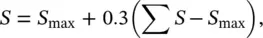
where S maxis the maximum loudness index and ∑ S is the sum of all the loudness indices. The 0.3 constant (used for octave bands) in Eq. (4.2)is replaced by 0.15 for one‐third‐octave bands. The Zwicker method is based on the critical band concept and, although more complicated than the Stevens method, can be used either with diffuse or frontal sound fields. Complete details of the procedures are given in the ISO standard [15] and Kryter [16] has discussed the critical band concept in his book.
Example 4.3
The octave band sound pressure levels (see column 2 of Table 4.1) of the noise from machines in a factory are given for the center frequencies (see column 1 of Table 4.1). Calculate the loudness level.
Solution
From Figure 4.8the loudness indices, S , given in column 3 of Table 4.1are found.
We obtain that S max= 26.5 and ∑ S = 134.2. Thus from Eq. (4.2)the loudness is: S = 26.5 + 0.3 (134.2 − 26.5) = 59 sones (OD, Octave Diffuse) and from Eq. (4.1), or Figure 4.7, the loudness level is: P = 99 phons (OD).
Table 4.1 Octave band levels of factory noise and Stevens' loudness indices.
| Octave band center frequency, Hz | Octave band level, dB | Band loudness index S |
|---|---|---|
| 31.5 | 75 | 3.0 |
| 63 | 79 | 6.2 |
| 125 | 82 | 10.5 |
| 250 | 85 | 15.3 |
| 500 | 85 | 18.7 |
| 1000 | 87 | 26.5 |
| 2000 | 82 | 23.0 |
| 4000 | 75 | 17.5 |
| 8000 | 68 | 13.5 |
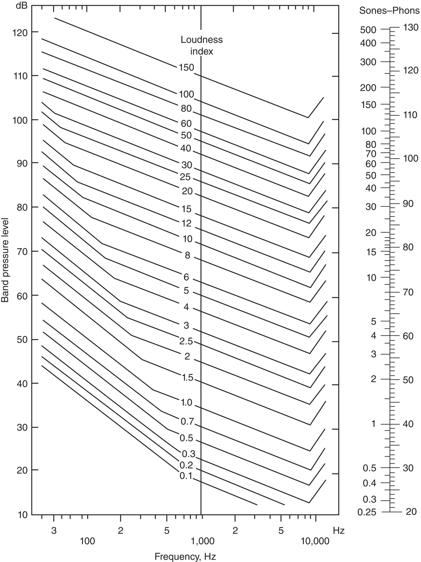
Figure 4.8 Contours of equal loudness index.
There are several other aspects of loudness which we have not had room to discuss in this book, e.g. impulsive noise, and monaural and binaural loudness. Readers will find these well covered in Kryter's book [16].
4.3.3 Masking
The masking phenomenon is well known to most people. A loud sound at one frequency can cause another quieter sound at the same frequency or a sound close in frequency to become inaudible. This effect is known as masking . Broadband sounds can have an even more complicated masking effect and can mask louder sounds over a much wider frequency range than narrow‐band sounds. These effects are important in human assessment of product sound quality.
Noise that contains pure tones is generally annoying and unpleasant. In the case of automobile interior noise, engine and exhaust system noise consists mostly of fundamental pure tones together with integer multiplies and broadband engine combustion noise. Similarly cooling fan noise consists of pure tones and broadband aerodynamic fan noise. In the case of automobiles, exhaust and cooling fan noise have some strong pure tone components. Wind noise and tire noise are mostly broadband in nature and can mask some of the engine, exhaust, and cooling fan noise, particularly at high vehicle speed. Figure 4.9shows the masking effect of broadband white noise. The solid lines represent the sound pressure level of a pure test tone (given in the ordinate) that can just be heard when the masking sound is white noise at the level shown on each curve. For example, it is seen that white noise at 40 dB masks pure tones at about 55 dB at 100 Hz, 60 dB at 1000 Hz, and 65 dB at 5000 Hz.
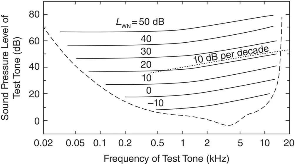
Figure 4.9 Contours joining sound pressure levels of pure tones at different frequencies that are masked by white noise at the spectral density level L WNshown on each contour [17, 18].
The masking of noise has been studied extensively for more than 70 years. The curves in Figure 4.9[17, 18] are very similar to those of much earlier research work by Fletcher and Munson in 1950 but are shown here since they have been extended to lower and higher frequencies than these earlier published results [19]. One interesting fact is that the curves shown in Figure 4.9are all almost parallel and are separated by about 10‐dB intervals, which is also the interval between the masker levels. This suggests that the masking of noise is almost independent of level at any given frequency. This fact was also established by Fletcher and Munson in 1950 as is shown in Figure 4.10[20]. Here the amount of masking is defined to be the upward shift in decibels in the baseline hearing threshold caused by the masking noise [19]. Figure 4.9shows that once the masker has reached a sufficient level to become effective, the amount of masking attained is a linear function of the masker level. This means, for instance, that a 10‐dB increase in the masker level causes a 10‐dB increase in the masked threshold of the signal being masked. It was found that this effect is independent of the frequency of the tone being masked and applies both to the masking of pure tones and speech [19, 20].
Figure 4.10 Masking of tones by noise at different frequencies and sound pressure levels [20].
Source: Reprinted with permission from [20], American Institute of Physics.
Figure 4.11shows the masking effect of a narrow‐band noise of bandwidth 160 Hz centered at 1000 Hz. The curves in Figure 4.11join the sound pressure levels of test tones that are just masked by the 1000‐Hz narrow‐band noise at the sound pressure level shown on each curve. It is observed that the curves are symmetric around 1000 Hz for low levels of the narrow‐band noise, while for high levels, the curves become asymmetric. It is seen that high levels of the narrow band of noise mask high‐frequency tones much better than low‐frequency tones. Figures 4.9and 4.11show that using either white noise or narrow‐band noise it is more difficult to mask low‐frequency than high‐frequency sounds. This fact is of some importance in evaluating the sound quality of a product since it is of no use to reduce or change the noise in one frequency range if it is masked by the noise at another frequency. There are other masking effects that are not normally as important for sound quality evaluations as the frequency effects discussed so far but still need to be described [16–19, 21–30].
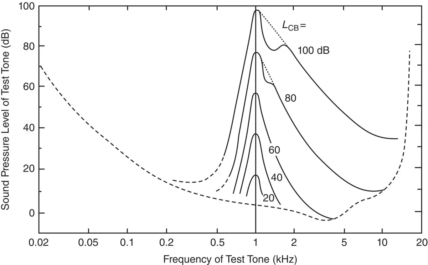
Figure 4.11 Masking effect of a narrow‐band noise of bandwidth 160 Hz centered at 1000 Hz. The contours join sound pressure levels of pure tones that are just masked by the 1000‐Hz narrow‐band noise at the sound pressure level shown on each contour [17, 18].
Читать дальшеИнтервал:
Закладка:
Похожие книги на «Engineering Acoustics»
Представляем Вашему вниманию похожие книги на «Engineering Acoustics» списком для выбора. Мы отобрали схожую по названию и смыслу литературу в надежде предоставить читателям больше вариантов отыскать новые, интересные, ещё непрочитанные произведения.


Обсуждение, отзывы о книге «Engineering Acoustics» и просто собственные мнения читателей. Оставьте ваши комментарии, напишите, что Вы думаете о произведении, его смысле или главных героях. Укажите что конкретно понравилось, а что нет, и почему Вы так считаете.