Malcolm J. Crocker - Engineering Acoustics

The sine and cosine terms in Eq. (1.1)can have values of the subscript n equal to 1, 2, 3, …, ∞. Hence, the signal x ( t ) will be made up of a fundamental frequency ω and multiples, 2, 3, 4, …, ∞ times greater. The A 0/2 term represents the D.C. (direct current) component (if present). The n th term of the Fourier series is called the n th harmonic of x ( t ). The amplitude of the n th harmonic is

(1.4)

and its square, 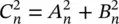, is sometimes called energy of the n th harmonic. Thus, the graph of the sequence is called the energy spectrum of x ( t ) and shows the amplitudes of the harmonics.

Buzz‐saw noise is commonly generated by supersonic fans in modern turbofan aircraft engines. A buzzing sound can be represented by the periodic signal shown in Figure 1.3. Find the Fourier series and the energy spectrum for this signal.

We are required to represent x ( t ) = At over the interval 0 ≤ t ≤ 1, T = 1, and the fundamental frequency is ω = 2 π / T = 2 π . Then, we determine the corresponding Fourier coefficients using Eqs. (1.3a)and (1.3b)

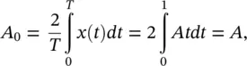
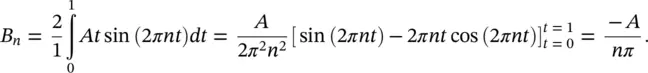
Therefore, substituting for the Fourier coefficients in Eq. (1.1)we get

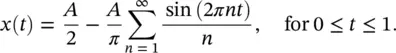
The energy spectrum of x ( t ) is shown in Figure 1.4. For this case the frequency spectrum is discrete, described by the Fourier coefficients ( Eq. (1.4)). Note that for a Fourier series with only sine terms, as in Example 1.1, the amplitude of the n th harmonic is C n= | B n|. The energy spectrum has spikes at multiples of the fundamental frequency (harmonics) with a height equal to the value of . Thus, the spectrum is a series of spikes at the frequencies ω = 2 πf , and overtones 2 ω = 2 × 2 πf , 3 ω = 3 × 2 πf , … with amplitudes ( A / π ) 2, ( A /2 π ) 2, ( A /3 π ) 2, … respectively.

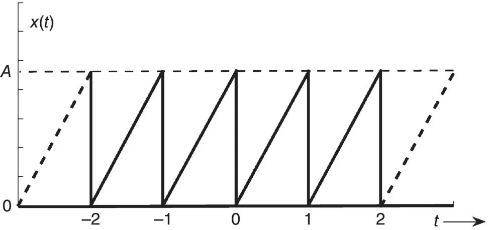
Figure 1.3 Periodic sound signal.

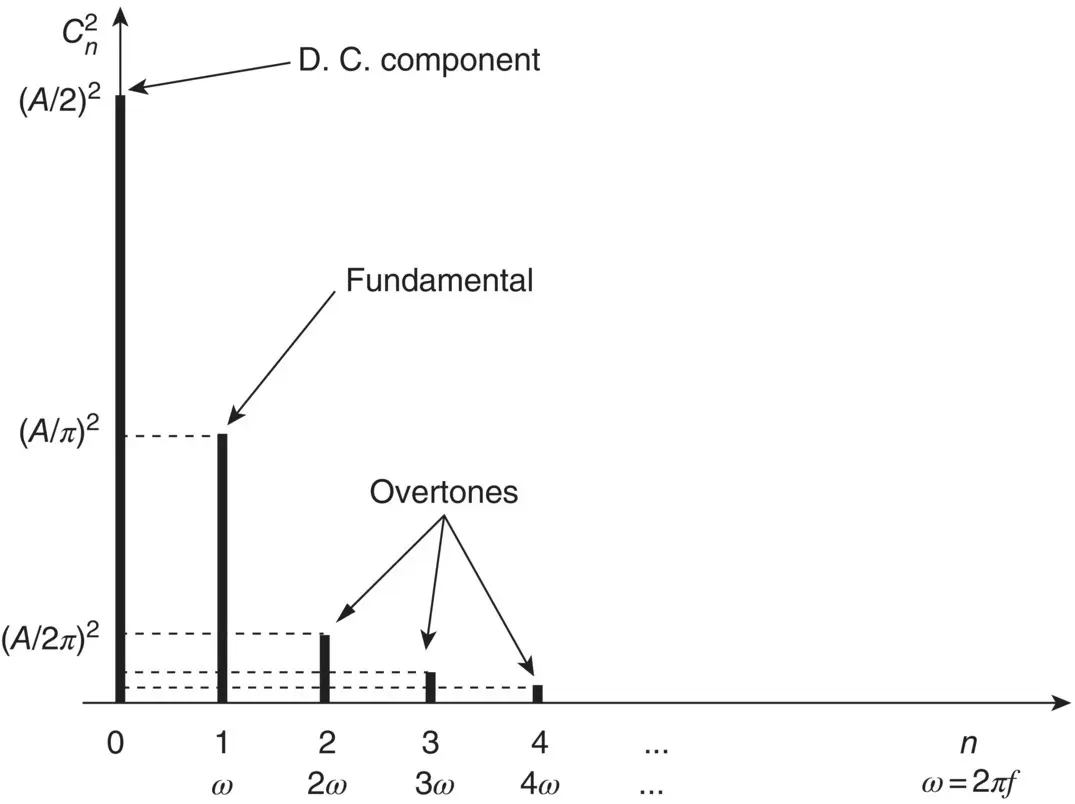
Figure 1.4 Frequency spectrum of the periodic signal of Figure 1.3.

Equation (1.1)is known as a Fourier series and can only be applied to periodic signals. Very often a sound signal is not a pure or a complex tone but is impulsive in time. Such a signal might be caused in practice by an impact, explosion, sonic boom, or the damped vibration of a mass‐spring system (see Chapter 2of this book) as shown in Figure 1.2c. Although we cannot find a Fourier series representation of the wave in Figure 1.2c because it is nonperiodic (it does not repeat itself), we can find a Fourier spectrum representation since it is a deterministic signal (i.e. it can be predicted in time). The mathematical arguments become more complicated [1, 7, 9] and will be omitted here. Briefly, the Fourier spectrum may be obtained by assuming that the period of the motion, T , becomes infinite. Then since f = ω /2 π = 1/ T , the fundamental frequency approaches zero and Eq. (1.2)passes from a summation of harmonics to an integral:

(1.5)

Just as C nwas complex in Eq. (1.2), X( ω ) is complex in Eq. (1.5), having both a magnitude and a phase. The Fourier spectrum (magnitude), ∣ X( ω )∣, of the wave in Figure 1.2c is plotted to the right of Figure 1.2c. ∣ X( ω )∣may be thought of as the amplitude of the time signal at each value of frequency ω .

So far we have discussed periodic and nonperiodic signals. In many practical cases the sound or vibration signal is not deterministic (i.e. it cannot be predicted) and it is random in time (see Figure 1.5). For a random signal, x ( t ), mathematical descriptions become difficult since we have to use statistical theory [1, 7, 9]. Theoretically, for random signals the Fourier transform X( ω ) does not exist unless we consider only a finite sample length of the random signal, for example, of duration τ in the range 0 < t < τ . Then the Fourier transform is

(1.6)

where X( ω , τ ) is the finite Fourier transform of x ( t ). Note that X( ω ) is defined for both positive and negative frequencies. In the real world x ( t ) must be a real function, which implies that the complex conjugate of Xmust satisfy X(− ω ) = X *( ω ); i.e. X( ω ) exhibits conjugate symmetry. Finite Fourier transforms can easily be calculated with special analog‐to‐digital computers (see Section 1.5).

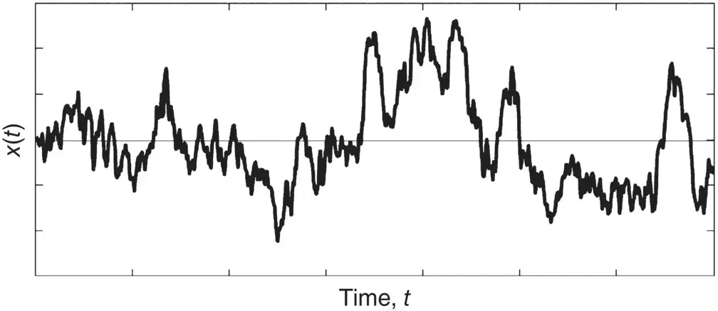
Figure 1.5 Random noise signal.

An R–C (resistance–capacitance) series circuit is a classic first‐order low‐pass filter (see Section 1.4). Transient response describes how energy that is contained in a circuit will become dissipated when no input signal is applied. The transient response of an R–C series circuit (for t > 0) is given by