Gregory T. Benz - Agitator Design for Gas-Liquid Fermenters and Bioreactors

When an impeller operates in turbulent flow, the loads on each blade are fluctuating about a mean. To better visualize this, imagine riding along in a car with your hand outside the window. You will note that your hand is buffeted about, with a highly variable force. This is due to turbulence, involving various shedding of vortices, etc. The same thing happens to an impeller in turbulent flow. The load on each blade varies with time, and the loads on each blade are not synchronous with each other. The result is that there will be a fluctuating net side load on the impeller, creating a bending load on the shaft. This load, sometimes called an imbalanced hydraulic force, is not due to mechanical imbalance or any lack of manufacturing precision. It is entirely due to the nature of turbulence.

The dimensionless hydraulic force equals the product of hydraulic force times impeller diameter divided by impeller torque:

(3.12)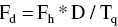

Normally, the peak value of this ratio is correlated, so that a peak value of hydraulic force may be predicted and used in shaft and impeller design. This group is a function of Reynolds number and impeller type, as well as geometric ratios, aeration number, and Froude number, and direction of pumping for axial flow impellers.

This relates impeller thrust to impeller parameters and density:

(3.13)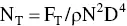

It is primarily used to determine impeller thrust for mechanical purposes. It also is used to predict cavern size for shear‐thinning fluids, as will be discussed in Chapter 12. Qualitatively, it is a constant in laminar and turbulent flow, but goes through a minimum in transition flow.

Figure 3.4represents a typical log/log plot of Power number as a function of Reynolds number, with D/T as a parameter. (The D/T effect is primarily noticeable on axial impellers. Radial impellers show much less dependency on D/T, as we will see in Chapter 5.)

Examining this curve, we can observe several things. One is that the power number becomes constant for a given D/T under turbulent conditions, i.e. at high Reynolds numbers (typically, above 20 000). When a manufacturer of an impeller states it power number, it is normally the turbulent power number at a D/T of 1/3 and a C/T of 1/3. Axial impellers will tend to have a decreasing power number at increasing D/T.

Also note that the curve becomes a 45° angle at laminar flow conditions (typically, N Re<10). That means the product of Reynolds number and Power number is constant in that range. A simple derivation reveals that in the laminar range,

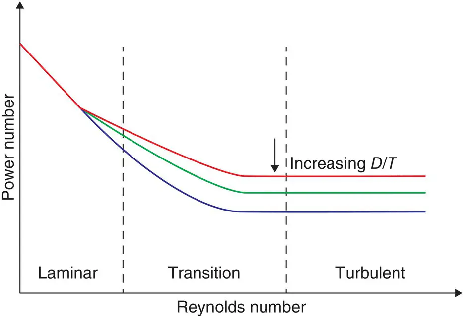
Figure 3.4 Typical power number curve.

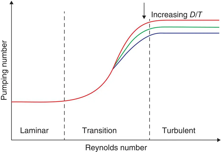
Figure 3.5 Typical pumping number curve.

(3.14)

The range between laminar and turbulent is called the transition range. It is a very broad range. That is because turbulence commences first near the impeller blade tips somewhere in the region of N Re= 10, but does not reach all of the far corners of the tank until N Re> 20 000. The power number gradually levels out in this range. For some impellers, it goes through a minimum in the transition range.

Figure 3.5represents a typical pumping number curve, as a function of Reynolds number and having D/T as a parameter.

In laminar flow, the pumping number becomes a constant. This means that under such conditions, the impeller pumping is independent of viscosity, though the power draw is directly proportional to viscosity.

In turbulent flow, the pumping number again becomes constant at a given D/T, though it is much higher than the laminar pumping number. As D/T increases, the pumping number generally decreases. This is because recirculating flow within the tank creates a velocity opposite the impeller discharge, impeding its flow. Nonetheless, larger impellers pump more for a given power input than smaller ones.

When vendors quote a pumping number, it is usually in turbulent flow and at a D/T of 1/3 and a C/T of 1/3. Many consider this geometry to be “standard”, but there is no fundamental reason to adhere to this geometry when designing agitation equipment.

Figure 3.6represents a typical generic blend time curve.

We can observe that blend time becomes constant in both laminar and turbulent flow. However, the laminar dimensionless blend time is often several orders of magnitude greater than the turbulent blend time. Specialized impellers have been developed for laminar flow mixing. We need not delve into these in this book, as fermenters never operate in the laminar range, because it is basically impossible to both incorporate gas into highly viscous liquids and have the gas exit in a reasonable amount of time after the gas is depleted.

Some versions of the dimensionless blend time curve incorporate the D/T effect into the Y‐axis expression, as stated under the dimensionless blend time definition given earlier.

Figure 3.7depicts gassing factor as a function of Aeration number for three different impeller types.

Gassing factor depends on Aeration number, Froude number, D/T, Reynolds number, and impeller type. Therefore, it is impossible to show the entire relationship on a simple two dimensional graph. Figure 3.7is based on turbulent flow, a D/T of 1/3, and a Froude number of 0.5.

We can readily see that the traditional impeller for gas dispersion, the Rushton (or disk) turbine, has a rather severe drop in power at high gas flow rates. As we will see later, this is a problem for maintaining maximum mass transfer. That is why it has been pretty much replaced by modern, deeply concave impellers such as the BT‐6 by Chemineer, the Phasejet by Ekato, and several others that have less effect of gas flow on power draw.

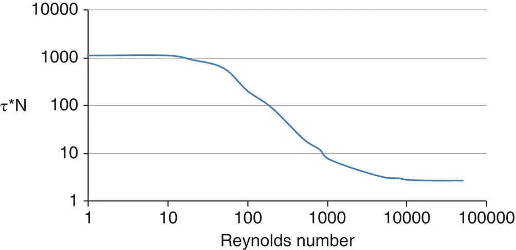
Figure 3.6 Dimensionless blend time.

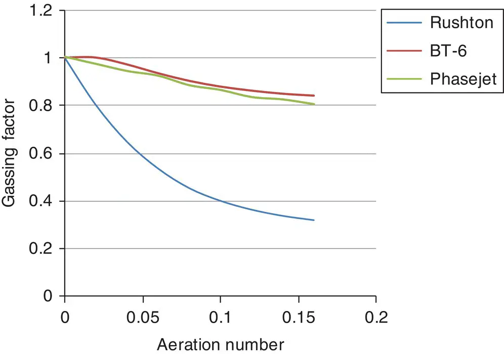
Figure 3.7 Gassing factors.

We will cover other dimensionless parameters, such as for heat transfer, as needed in subsequent chapters. For now, we will show some example calculations.

A tank has an impeller of 1000 mm diameter, rotating at a shaft speed of 125 rpm, in a fluid with a specific gravity of 1.2. It has a known power number of 0.75. How much power will it draw?

It is best to first convert all parameters to SI units. So, we have a 1m impeller diameter, turning at a shaft speed of 125 rpm/60, or 2.0833/s, in a fluid with a density of 1200 kg/m 3. Since the power number is dimensionless, it remains at 0.75. The definition of power number, from Eq. 3.3, is: